Hyperbola summation refined into the Kirchhoff method

Schneider [1978] states the analytic representation for the Huygens secondary wavelet  

$$\hbox{FT}^{-1} ( e^{{i} \, k_z \, z } ) \quad =\quad {1 \ove... ...{\rm step} ( t \,-\, r/v ) \over \sqrt{ t^2 \,-\, r^2 / v^2 }}$$ (19)

where r is the distance $\sqrt{ x^2 \,+\, (z-z_0 )^2 }$ between the (exploding reflector) source and the receiver. The function (19) contains a pole and the derivative of a step function. Because of the infinities it really cannot be graphed. But from the mathematical form you immediately recognize that the disturbance concentrates on the expected cone. The derivative of the step function gives a positive impulsive arrival on the cone. The derivative of the inverse square root gives the impulse a tail of negative polarity decaying with a -3/2 power. The cosine obliquity arises because the derivative is a z derivative and not an r derivative.

Equation (19) states the two -dimensional Huygens wavelet, not the three -dimensional wavelet (which differs in some minor aspects). Although waves from point sources are mainly spherical, the focusing of bent layers is mainly a two-dimensional focusing, i.e., bent layers are more like cylinders than spheres.

You might wonder why anyone would prefer approximations, given the exact inverse transform (19). The difficulty of graphing (19) shows up in practice as a difficulty in convolving it with data. That is why early Kirchhoff migrations were generally recognizable by precursor noise above a flat sea floor. Chapters , , and , are largely devoted to extensions of (19) that are valid with variable velocity and that are better representations on a data mesh.

In the Fourier domain, the Huygens secondary source function is simple and smooth. It is a straightforward matter to evaluate the function on a rectangular mesh and inverse transform with ft1axis() and ft2axis() . Figure 8 shows the result on a 256 $\times$ 64 point mesh.

 

huygens
Figure 8 The Huygens wavelet (top) and a smoothed time integral (bottom).

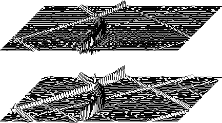(In practice the mesh would be about 1024 $\times$ 256 or more, but the coarser mesh used here provides a plot of suitable detail). Because of the difficulty in plotting functions that resemble an impulsive doublet, a second plot of the time integral, (with gentle band limiting) is displayed in the lower part of Figure 8.