SUMMATION AND SUPERPOSITION OF CONICS

The methods of hyperbola summation and semicircle superposition are the most comprehensible of all known methods.

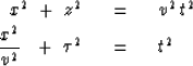
Recall the equation for a conic section, that is, a circle in (x,z)-space or a hyperbola in (x,t)-space. Converting to travel-time depth $\tau$

$$\begin{eqnarray} x^2 \ +\ z^2 \ \ &=&\ \ v^2 \, t^2 \\ { x^2 \over v^2 } \ \ +\ \tau^2 \ \ &=&\ \ t^2\end{eqnarray}$$ (17) (18)

Figure 6, which is from Schneider's classic paper [1971], illustrates the semicircle-superposition method.

 

schneider
Figure 6 The process may be described in numerous ways. Two very simple and equally valid representations are indicated in Figures 6 and 7. Shown here is a representation of the process in terms of what happens to a single input trace plotted in depth (time may also be used) midway between its source and receiver. Each amplitude value of this trace is mapped into the subsurface along a curve representing the loci of points for which the travel time from source to reflection point to receiver is constant. If the velocity is constant, these curves are ellipses with source and receiver as foci. The picture produced by this operation is simply a wavefront chart modulated by the trace amplitude information. This clearly is not a useful image in itself, but when the map is composited with similar maps from neighboring traces (and common-depth-point traces of different offsets), useful subsurface images are produced by virtue of constructive and destructive interference between wavefronts in the classical Huygens sense. For example, wavefronts from neighboring traces will all intersect on a diffraction source, adding constructively to produce an image of the diffractor as a high-amplitude blob whose (z,x) resolution is controlled by the pulse bandwidth and the horizontal aperture of the array of neighboring traces composited. For a reflecting surface, on the other hand, wavefronts from adjacent traces are tangent to the surface and produce an image of the reflector by constructive interference of overlapping portions of adjacent wavefronts. In subsurface regions devoid of reflecting and scattering bodies, the wavefronts tend to cancel by random addition. (figure and caption from Schneider, W. A., 1971 [by permission])

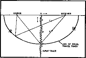Taking the data field to contain a few impulse functions, the output should be a superposition of the appropriate semicircles. Each semicircle denotes the spherical-reflector earth model that would be implied by a dataset with a single pulse. Taking the data field to be one thousand seismograms of one thousand points each, then the output is a superposition of one million semicircles. Since a seismogram has both positive and negative polarities, about half the semicircles will be superposed with negative polarities. The resulting superposition could look like almost anything. Indeed, the semicircles might mutually destroy one another almost everywhere except at one isolated impulse in $(x, \tau$)-space. Should this happen you might rightly suspect that the input data section in (x,t)-space is a Huygens secondary source, namely, energy concentrated along a hyperbola. This leads us to the hyperbola-summation method.

The hyperbola-summation method of migration is depicted in Figure 7.

 

schneider2 Figure 7 A second description of the process is provided here. The process is represented in terms of how an output trace is developed from an ensemble of input traces, shown as CDP-stacked traces in the upper half of the figure. The output in the lower half reflects how each amplitude value at (x,z) is obtained by summing input amplitudes along the travel-time curve shown. This curve defines a diffraction hyperbola. If a diffraction source existed in the subsurface at the output point shown, then a large amplitude would result. The process also works for reflectors since a reflector may be regarded as a continuum of diffracting elements whose individual images merge to produce a smooth continuous boundary. (figure and caption from Schneider, 1971)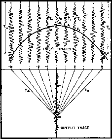

The idea is to create one point in $(x, \tau )$-space at a time, unlike in the semicircle method, where each point in $(x, \tau )$-space is built up bit by bit as the one million semicircles are stacked together. To create one fixed point in the output $(x, \tau$)-space, imagine a hyperbola, equation (18), set down with its top on the corresponding position of (x,t)-space. All data values touching the hyperbola are added together to produce a value for the output at the appropriate place in $(x, \tau$)-space. In the same way, all other locations in $(x, \tau$)-space are filled. We can wonder whether the hyperbola-migration method is better or worse than or equivalent to the semicircle method.

The opposite of data processing or building models from data is constructing synthetic data from models. With a slight change, the above two processing programs can be converted to modeling programs. Instead of hyperbola summation or semicircle superposition, you do hyperbola superposition or semicircle summation. We can also wonder whether the processing programs really are inverse to the modeling programs. Some factors that need to be considered are (1) the angle-dependence of amplitude (the obliquity function) of the Huygens waveform, (2) spherical spreading of energy, and (3) the phase-shift on the Huygens waveform. It turns out that results are reasonably good even when these complicating factors are ignored.

As other methods of migration were developed, the deficiencies of the earlier methods were more clearly understood and found to be largely correctable by careful implementation. One advantage of the later methods is that they implement true all-pass filters. Such migrations preserve the general appearance of the data. This suggests restoration of high frequencies, which tend to be destroyed by hyperbolic integrations. Work with the Kirchhoff diffraction integral by Trorey [1970] and Hilterman [1970] led to forward modeling programs. Eventually (Schneider [1977]) this work suggested quantitative means of bringing hyperbola methods into agreement with other methods, at least for constant velocity. Common terminology nowadays is to refer to any hyperbola or semicircular method as a Kirchhoff method, although, strictly speaking, the Kirchhoff integral applies only in the constant-velocity case.