Seismic imaging is the numerical process of creating
an image of the subsurface from
reflections recorded at the surface.
The recorded data sets are made of an ensemble of time series (
seismic traces).
The amplitude of the signal is
proportional to the pressure (or particle velocity) at the location
of each receiver.
The seismic waves are generated by artificial sources
(
controlled sources).
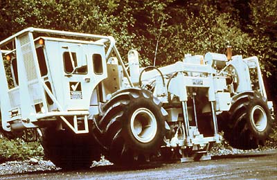
On land, the sources are either dynamite explosions
or vibrator trucks (
vibroseises),
and the receivers are geophones planted in the ground.
The image on the left shows a vibroseis truck in action.
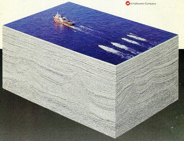
Marine data sets are recorded by specially built vessels that
pull several (up to 12) long (4 to 10 kilometers) streamers
with hydrophones every 5 meters.
The seismic sources are placed at the stern of the boat.
They are called air-guns and are essentially
compressors that release huge air bubbles in the water.
The panel on the right shows a seismic vessel in action.
Chapter 1
in
3-D Seismic Imaging
discusses current acquisition practices and geometries.
We can gain an intuitive understanding of the reflection seismic experiment
by observing the wave-propagation movie shown below.
The image on the left shows the simple reflectivity model assumed
in the subsurface:
a shallower dipping reflector and a deeper flat reflector.
These reflectors are respectively marked by the cyan and yellow lines in
the movie displayed in the panel in the middle.
The image on the right shows the data collected at the
surface by this simple numerical experiment (shot profile).
The time axis is vertical and represents the traveltime
of the recorded reflections.
The horizontal axis is the distance from the source location (offset).
As expected, the traveltimes of the reflections
are longer as the receivers are further from the source.
Notice that the traveltime curve from the flat reflector
is symmetric around zero offset and is an ``exact'' hyperbola,
whereas the traveltime curve from the dipping reflector
is not symmetric.
Seismic imaging can be seen as the inverse process of the seismic experiment.
Indeed, seismic migration, the most common method
to image seismic data, can be mathematically defined as an approximation of
the inverse of the linear operator (modeling operator)
that links the reflectivity model
(on the left above)
to the recorded data
(on the right above).
Migration is
frequently
defined as the simplest possible approximation
of the inverse of the modeling operator; that is, its adjoint.
Surprisingly, this seemingly crude approximation is successful to image
the shape of the reflectors in the most of practical situations.
It fails only when the reflectors are not well illuminated
either because of insufficient data coverage or
because complex overburden substantially distorts the wavefields.
You can learn more about the challenges to produce good images in these
situations in
Chapter 8
and
Chapter 9
in
3-D Seismic Imaging.
The movie below illustrates the migration process
as the time reversal of the modeling process.
This particular method for imaging
seismic data is called
reverse-time migration
(see
Chapter 4
in
3-D Seismic Imaging
).
Reverse-time migration is seldom used in practice
but it leads to an intuitive conceptual
understanding of the general concept of migration.
The panel on the left shows the propagation
of the source wavefield backward in time;
notice that the wavefront collapse toward the source instead of
expanding away from it.
The panel in the middle shows the reverse propagation
of the receiver wavefield, using the recorded
shot profile as a time-dependent boundary condition at the
top of the computational domain.
The data are injected backward in time starting from the last time sample
in the data traces.
The panel on the right shows the image as it is created
by the application of the imaging condition
to the two propagating wavefields.
In this case, the imaging condition is the extraction
of the zero-time lag of the cross-correlation of the two
wavefields.