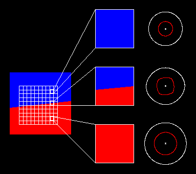
Figure 1: (GIF) (PS) Left: A sampling grid laid down on a medium made up of two homogeneous blocks. Three representative grid cells have been highlighted. Center column: Expanded views of the three representative grid cells. Right column: P-SV impulse responses of the homogeneous equivalent medium for each expanded grid cell.
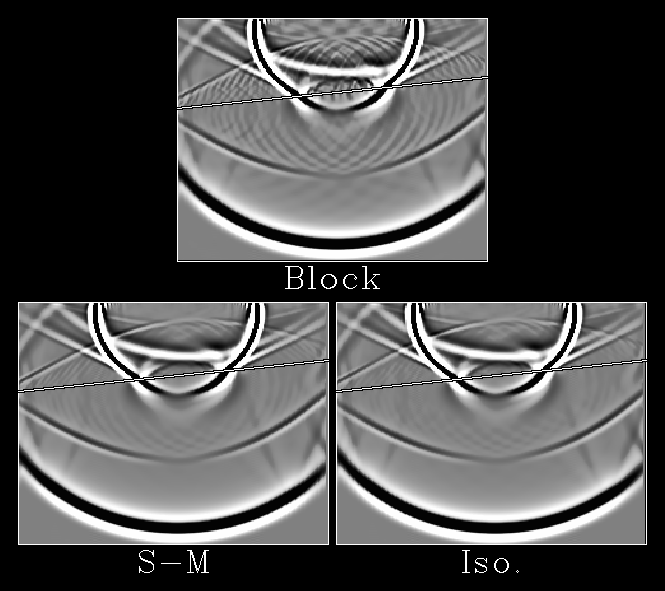
Figure 2: (GIF) (PS) Snapshots comparing the results of a wavefield hitting a gently sloping reflector for three similar models. The only difference is in how the sloped boundary was represented on the discrete computational grid. In the top plot nearest neighbor interpolation was used; the boundary comes out as a series of flat stretches with a stair step every 10 grid cells. The steps cause noticeable diffractions that would not be present in an ideal continuum model. In the bottom left plot S-M interpolation was used; in the bottom right plot the isotropic P and S slownesses were interpolated independently. Both these methods mostly avoid the unwanted diffractions. (The primaries are strongly clipped so that the weaker converted waves and diffractions can be seen.)
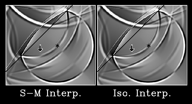
Figure 3: (GIF) (PS) Snapshots comparing the results of a wavefield hitting a 45-degree sloping reflector for two similar models. In the left plot S-M interpolation was used; in the right plot isotropic slowness averaging was used. The arrow points out where the reflected S wave would have a zero crossing in the ideal continuum case. S-M interpolation on the discrete grid correctly reproduces the zero crossing, while isotropic slowness averaging approximates the sign change with a gradual phase shift.