|
filter
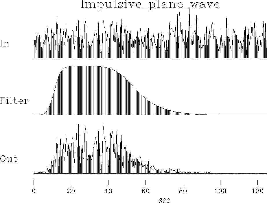
Figure 7 Random numbers into a filter. Top is a spectrum of random numbers. Middle is the spectrum of a filter. Bottom is the spectrum of filter output. |  |
|
filter
Figure 7 Random numbers into a filter. Top is a spectrum of random numbers. Middle is the spectrum of a filter. Bottom is the spectrum of filter output. |  |
From the spectrum of the output we can guess the spectrum of the filter, but the figure shows there are some limitations in our ability to do so. Let us analyze this formally.
Observations of sea level over a long period of time
can be summarized in terms of a few statistical averages,
such as the mean height m and the variance ![]() .Another important kind of statistical average
for use on geophysical time series
is the
``power spectrum."
Many mathematical models
explain only statistical averages of data and not the data itself.
To recognize certain pitfalls
and understand certain fundamental limitations
on work with power spectra,
we first consider the idealized example of random numbers.
.Another important kind of statistical average
for use on geophysical time series
is the
``power spectrum."
Many mathematical models
explain only statistical averages of data and not the data itself.
To recognize certain pitfalls
and understand certain fundamental limitations
on work with power spectra,
we first consider the idealized example of random numbers.
 |
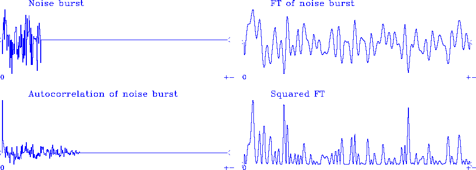
Figure 8 shows a signal that is a burst of noise; its Fourier transform, and the transform squared; and its inverse transform, the autocorrelation. Here the FT squared is the same as the more usual FT times its complex conjugate--because the noise-burst signal is even, its FT is real.
Notice that the autocorrelation has a big spike at zero lag. This spike represents the correlation of the random numbers with themselves. The other lags are much smaller. They represent the correlation of the noise burst with itself shifted. Theoretically, the noise burst is not correlated with itself shifted: these small fluctuations result from the finite extent of the noise sample.
Imagine many copies of Figure 8. Ensemble averaging would amount to adding these other autocorrelations or, equivalently, adding these other spectra. The fluctuations aside the central lobe of the autocorrelation would be destroyed by ensemble averaging, and the fluctuations in the spectrum would be smoothed out. The expectation of the autocorrelation is that it is an impulse at zero lag. The expectation of the spectrum is that it is a constant, namely,
| (35) |