

Next: References
Up: GEOMETRY-BASED DECON
Previous: A model for convolution
In Figure 6, we can see
that events remain which look suspiciously like multiple reflections.
Careful inspection of the data (rapid blinking on a video screen)
convinced me that the problem lay in imperfect modeling
of depth-variable velocity.
It is not enough to use a depth-variable velocity in the NMO
(a constant velocity was used in Figure 6), because
primary and multiple reflections have different velocities
at the same time.
I used instead a physical technique called ``diffraction"
(explained in detail in IEI)
to make the regressors.
Instead of simply shifting on the time axis,
diffraction shifts on the depth axis,
which results in subtle changes in hyperbola curvature.
veld
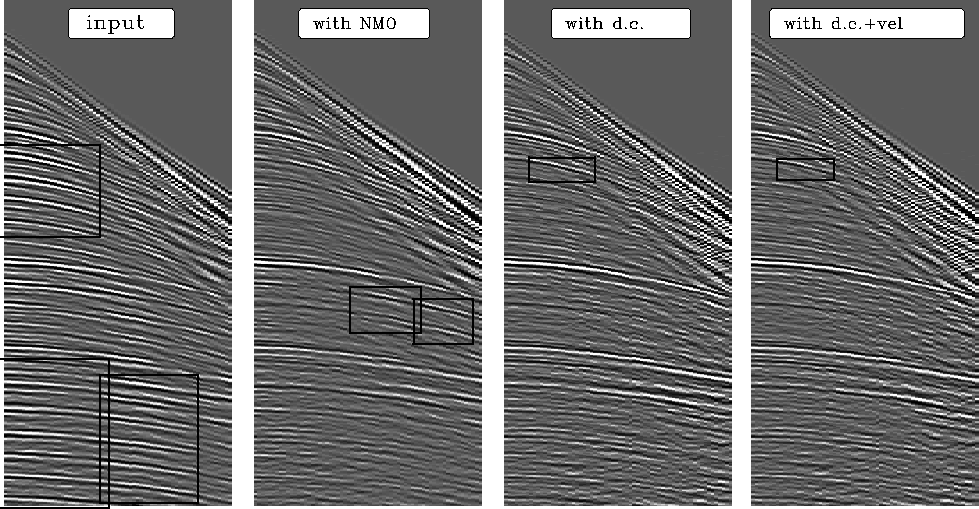
Figure 9
Left is the original data.
Next is the result of using NMO in the regressors.
Next, the result of downward continuation in the regressors.
On the right, velocity scans were also used.
Rectangles outline certain or likely multiple reflections.

The downward-continuation result is significantly better than
the NMO result,
but it does contain some suspicious reflections (boxed).
My final effort, shown on the right, includes the idea
that the data contains random noise which could be windowed away
in velocity space.
To understand how this was done,
recall that the basic model is
 , where
 is the left panel,
 are constants determined by least squares,
and
  are the regressors, which
are panels like
  but delayed and diffracted.
Let
  denote an operator that transforms to velocity space.
Instead of solving the regression
 ,I solved the regression
 and used the resulting values of
  in the original (t,x)-space.
(Mathematically, I did the same thing when making
Figure
 ![[*]](http://sepwww.stanford.edu/latex2html/cross_ref_motif.gif) .)
This procedure offers the possible advantage that a weighting function
can be used in the velocity space.
Applying all these ideas,
we see that a reflector remains which looks
more like a multiple than a primary.
.)
This procedure offers the possible advantage that a weighting function
can be used in the velocity space.
Applying all these ideas,
we see that a reflector remains which looks
more like a multiple than a primary.
A proper ``industrial strength'' attack on multiple reflections
involves all the methods discussed above,
wave-propagation phenomena described in IEI,
and judicious
averaging in the space of source and receiver distributions.


Next: References
Up: GEOMETRY-BASED DECON
Previous: A model for convolution
Stanford Exploration Project
10/21/1998

![[*]](http://sepwww.stanford.edu/latex2html/cross_ref_motif.gif)