


A rich literature (c.f. FGDP) exists on the one-dimensional model of multiple reflections. Some authors develop many facets of wave-propagation theory. Others begin from a simplified propagation model and develop many facets of information theory. These one-dimensional theories are often regarded as applicable only at zero offset. However, we will see that all other offsets can be brought into the domain of one-dimensional theory by means of slant stacking.
The way to get the timing and amplitudes of multiples
to work out like vertical
incidence is to stop thinking of seismograms as time functions
at constant offset, and start thinking of constant Snell parameter.
In a layered earth the complete raypath is constructed by summing
the path in each layer.
At vertical incidence ![]() , it is obvious that when
a ray is in layer j its travel time tj for that layer
is independent of any other layers which may also be traversed
on other legs of the total journey.
This independence of travel time
is also true for any other fixed p.
But, as shown in Figure 12, it is not true for a ray
whose total offset
, it is obvious that when
a ray is in layer j its travel time tj for that layer
is independent of any other layers which may also be traversed
on other legs of the total journey.
This independence of travel time
is also true for any other fixed p.
But, as shown in Figure 12, it is not true for a ray
whose total offset ![]() , instead of its p, is fixed.
, instead of its p, is fixed.
|
multangle
Figure 12 Rays at constant-offset (left) arrive with various angles and hence various Snell parameters. Rays with constant Snell parameter (right) arrive with various offsets. At constant p all paths have identical travel times. | 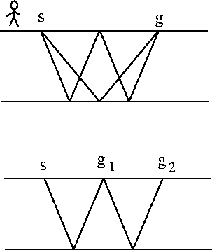 |

Likewise, for fixed p, the horizontal distance ![]() which
a ray travels while in layer j is independent
of other legs of the journey.
Thus, in addition,
which
a ray travels while in layer j is independent
of other legs of the journey.
Thus, in addition, ![]() const
const![]() for any layer j is
independent of other legs of the journey.
So
for any layer j is
independent of other legs of the journey.
So ![]() is a property of the
is a property of the ![]() layer and has nothing to do
with any other layers which may be in the total path.
Given the layers that a ray crosses,
you add up the tj and the fj for each layer,
just as you would in the vertical-incidence case.
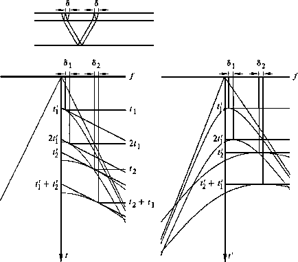
Some paths are shown in Figure 13.
layer and has nothing to do
with any other layers which may be in the total path.
Given the layers that a ray crosses,
you add up the tj and the fj for each layer,
just as you would in the vertical-incidence case.
Some paths are shown in Figure 13.
 |
To see how to relate field data to slant stacks,
begin by searching on a common-midpoint gather for all those
patches of energy (tangency zones) where the
hyperboloidal arrivals attain some particular
numerical value of slope ![]() .These patches of energy seen on the surface observations
each tell us where and when
some ray of Snell's parameter p has hit the surface.
Typical geometries and synthetic data are shown
in figures 13 and 14.
.These patches of energy seen on the surface observations
each tell us where and when
some ray of Snell's parameter p has hit the surface.
Typical geometries and synthetic data are shown
in figures 13 and 14.
Both the tj and the tj' behave like the times of normal-incident multiple reflections. While the lateral location of any patch unfortunately depends on the velocity model v(z), slant stacking makes the lateral location irrelevant. In principle, slant stacking could be done for many separate values of p so that the (f,t)-space would get mapped into a (p,t)-space. The nice thing about (p,t)-space is that the multiple-suppression problem decouples into many separate one-dimensional problems, one for each p-value. Not only that, but the material velocity is not needed to solve these problems. It is up to you to select from the many published methods. After suppressing the multiples you inverse slant stack. Once back in (f,t)-space you could estimate velocity and further suppress multiples using your favorite stacking method.
Figure 14 is a ``workbook'' exercise.
 |


By picking the tops of all events on the right-hand frame
and then connecting the picks with dashed lines,
you should be able to verify that sea-bottom peglegs
have the same interval velocity as the simple bottom multiples.
The interval velocity of the sediment can be measured from the primaries.
The sediment velocity can also be measured
by connecting the ![]() simple multiple
with the
simple multiple
with the ![]() pegleg multiple.
pegleg multiple.
Transformation to one dimension by slant stack for deconvolution is a process that lies on the border between experimental work and industrial practice. See for example Treitel et al [1982]. Its strength is that it correctly handles the angle-dependences that arise from the source-receiver geometry as well as the intrinsic angle-dependence of reflection coefficient. One of its weaknesses is that it assumes lateral homogeneity in the reverberating layer. Water is extremely homogeneous, but sediments at the water bottom can be quite inhomogeneous.