Signal/noise decomposition examples

filter ! multidip multidip filtering Figure  demonstrates the signal/noise decomposition concept on synthetic data. The signal and noise have similar frequency spectra but different dip spectra.

 

signoi90
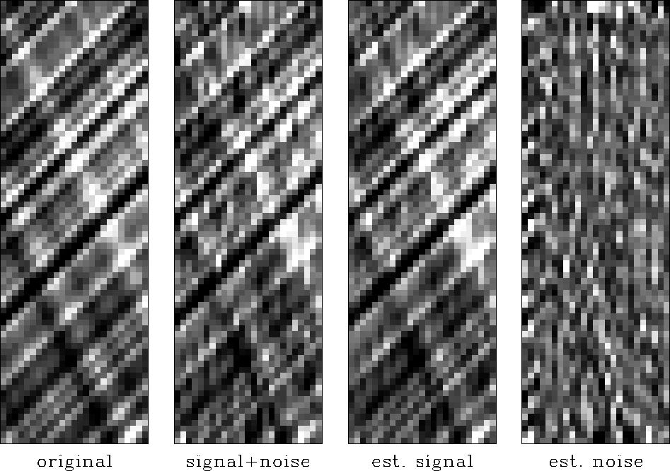
Figure 12 The input signal is on the left. Next is that signal with noise added. Next, for my favorite value of epsilon=1., is the estimated signal and the estimated noise.

Before I discovered helix preconditioning, Ray Abma found that different results were obtained when the fitting goal was cast in terms of $\bold n$ instead of $\bold s$.Theoretically it should not make any difference. Now I believe that with preconditioning, or even without it, if there are enough iterations, the solution should be independent of whether the fitting goal is cast with either $\bold n$ or $\bold s$.

Figure  shows the result of experimenting with the choice of $\epsilon$.As expected, increasing $\epsilon$weakens $\bold s$ and increases $\bold n$.When $\epsilon$ is too small, the noise is small and the signal is almost the original data. When $\epsilon$ is too large, the signal is small and coherent events are pushed into the noise. (Figure  rescales both signal and noise images for the clearest display.)

 

signeps90
Figure 13 Left is an estimated signal-noise pair where epsilon=4 has improved the appearance of the estimated signal but some coherent events have been pushed into the noise. Right is a signal-noise pair where epsilon=.25, has improved the appearance of the estimated noise but the estimated signal looks no better than original data.

Notice that the leveling operators $\bold S$ and $\bold N$ were both estimated from the original signal and noise mixture $\bold d = \bold s +\bold n$shown in Figure . Presumably we could do even better if we were to reestimate $\bold S$ and $\bold N$ from the estimates $\bold s$ and $\bold n$ in Figure .