 |
(1) |
![[*]](http://sepwww.stanford.edu/latex2html/cross_ref_motif.gif) to find the filter (1),
if we set up the
lag table lag
appropriately.
Then we could throw away alternate zeroed rows and columns (rescale the lag) to get the filter
to find the filter (1),
if we set up the
lag table lag
appropriately.
Then we could throw away alternate zeroed rows and columns (rescale the lag) to get the filter
| |
(2) |
![[*]](http://sepwww.stanford.edu/latex2html/cross_ref_motif.gif) ,
to find the interleaved data
because both
the filters (1) and (2)
have the same dip characteristics.
,
to find the interleaved data
because both
the filters (1) and (2)
have the same dip characteristics.
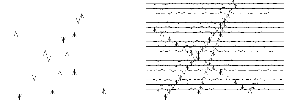
Figure ![[*]](http://sepwww.stanford.edu/latex2html/cross_ref_motif.gif) shows three plane waves recorded on five channels
and the interpolated data.
shows three plane waves recorded on five channels
and the interpolated data.
 |
Both the original data and the interpolated data can be described
as ``beyond aliasing,'' because on the input data
the signal shifts exceed the signal duration.
The calculation requires only a few seconds
of a two-stage least-squares method, in which the first stage
estimates a PEF (inverse spectrum) of the known data,
and the second uses the PEF to estimate the missing traces.
Figure ![[*]](http://sepwww.stanford.edu/latex2html/cross_ref_motif.gif) comes from PVI
which introduces the clever method described above.
We will review how that was done and examine the F90 codes
that generalize it to N-dimensions.
Then we'll go on to more general methods
that allow missing data in any location.
Before the methods of this section
are applied to field data for migration,
data must be broken into many overlapping tiles
of size about like those shown here
and the results from each tile pieced together.
That is described later in chapter
comes from PVI
which introduces the clever method described above.
We will review how that was done and examine the F90 codes
that generalize it to N-dimensions.
Then we'll go on to more general methods
that allow missing data in any location.
Before the methods of this section
are applied to field data for migration,
data must be broken into many overlapping tiles
of size about like those shown here
and the results from each tile pieced together.
That is described later in chapter ![[*]](http://sepwww.stanford.edu/latex2html/cross_ref_motif.gif) .
.
A PEF is like a differential equation.
The more plane-wave solutions you expect,
the more lags you need on the data.
Returning to Figure ![[*]](http://sepwww.stanford.edu/latex2html/cross_ref_motif.gif) ,
the filter must cover four traces (or more)
to enable it to predict three plane waves.
In this case,
na=(9,4).
As usual, the spike on the 2-D PEF is at
center=(5,1).
We see the filter is expanded by a factor of
jump=4.
The data size is
nd=(75,5)
and gap=0.
Before looking at the code
lace
,
the filter must cover four traces (or more)
to enable it to predict three plane waves.
In this case,
na=(9,4).
As usual, the spike on the 2-D PEF is at
center=(5,1).
We see the filter is expanded by a factor of
jump=4.
The data size is
nd=(75,5)
and gap=0.
Before looking at the code
lace ![[*]](http://sepwww.stanford.edu/latex2html/cross_ref_motif.gif) for estimating the PEF,
it might be helpful to recall the basic utilities
line2cart and
cart2line
for estimating the PEF,
it might be helpful to recall the basic utilities
line2cart and
cart2line
![[*]](http://sepwww.stanford.edu/latex2html/cross_ref_motif.gif) for conversion between a multidimensional space and
the helix filter lag.
We need to sweep across the whole filter
and ``stretch'' its lags on the 1-axis.
We do not need to stretch its lags on the 2-axis
because the data has not yet been interlaced by zero traces.
lacefill missing traces by rescaling PEF
The line ii(1)=ii(1)*jump
means we interlace the 1-axis but not the 2-axis because
the data has not yet been interlaced with zero traces.
For a 3-D filter
aa(na1,na2,na3),
the somewhat obtuse expression
(/na(1)*jump, na(2:)/)
is a three component
vector containing
(na1*jump, na2, na3).
for conversion between a multidimensional space and
the helix filter lag.
We need to sweep across the whole filter
and ``stretch'' its lags on the 1-axis.
We do not need to stretch its lags on the 2-axis
because the data has not yet been interlaced by zero traces.
lacefill missing traces by rescaling PEF
The line ii(1)=ii(1)*jump
means we interlace the 1-axis but not the 2-axis because
the data has not yet been interlaced with zero traces.
For a 3-D filter
aa(na1,na2,na3),
the somewhat obtuse expression
(/na(1)*jump, na(2:)/)
is a three component
vector containing
(na1*jump, na2, na3).
After the PEF has been found, we can get missing data in
the usual way with with module
mis2 ![[*]](http://sepwww.stanford.edu/latex2html/cross_ref_motif.gif) .
.