Kolmogoroff spectral factorization

With Fourier analysis we find a method of spectral factorization that is as fast as Fourier transformation, namely $N\log N$ for a matrix of size N. This is very appealing. An earlier version of this book included such an algorithm. Pedagogically, I didn't like it in this book because it requires lengthy off-topic discussions of Fourier analysis which are already found in both my first book FGDP and my third book PVI.

The Kolmogoroff calculation is based on the logarithm of the spectrum. The logarithm of zero is minus infinity -- an indicator that perhaps we cannot factorize a spectrum which becomes zero at any frequency. Actually, the logarithmic infinity is the gentlest kind. The logarithm of the smallest nonzero value in single precision arithmetic is about -36 which might not ruin your average calculation. Mathematicians have shown that the integral of the logarithm of the spectrum must be bounded so that some isolated zero values of the spectrum are not a disaster. In other words, we can factor the (negative) second derivative to get the first derivative. This suggests we will never find a causal bandpass filter. It is a contradiction to desire both causality and a spectral band of zero gain.

The weakness of the Kolmogoroff method is related to its strength. Fourier methods strictly require the matrix to be a band matrix. A problem many people would like to solve is how to handle a matrix that is ``almost'' a band matrix -- a matrix where any band changes slowly with location. Blind deconvolution A area of applications that leads directly to spectral factorization is ``blind deconvolution.'' Here we begin with a signal. We form its spectrum and factor it. We could simply inspect the filter and interpret it, or we might deconvolve it out from the original data. This topic deserves a fuller exposition, say for example as defined in some of my earlier books. Here we inspect a novel example that incorporates the helix.

 

solar
Figure 9 Raw seismic data on the sun (left). Impulse response of the sun (right) derived by Helix-Kolmogoroff spectral factorization.

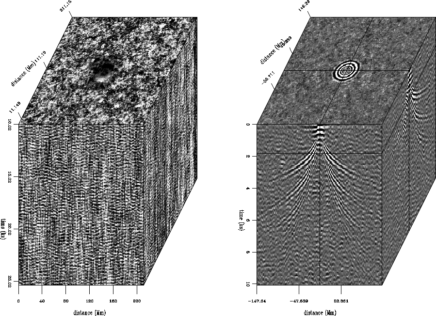
Solar physicists have learned how to measure the seismic field of the sun surface. If you created an impulsive explosion on the surface of the sun, what would the response be? James Rickett and I applied the helix idea along with Kolmogoroff spectral factorization to find the impulse response of the sun. Figure shows a raw data cube and the derived impulse response. The sun is huge so the distance scale is in megameters (Mm). The United States is 5 Mm wide. Vertical motion of the sun is measured with a video-camera like device that measures vertical motion by doppler shift. From an acoustic/seismic point of view, the surface of the sun is a very noisy place. The figure shows time in kiloseconds (Ks). We see about 15 cycles in 5 Ks which is 1 cycle in about 333 sec. Thus the sun seems to oscillate vertically with about a 5 minute period. The top plane of the raw data in Figure (left panel) happens to have a sun spot in the center. The data analysis here is not affected by the sun spot so please ignore it.

The first step of the data processing is to transform the raw data to its spectrum. With the helix assumption, computing the spectrum is virtually the same thing in 1-D space as in 3-D space. The resulting spectrum was passed to Kolmogoroff spectral factorization code. The resulting impulse response is on the right side of Figure . The plane we see on the right top is not lag time $\tau=0$;it is lag time $\tau=2$ Ks. It shows circular rings, as ripples on a pond. Later lag times (not shown) would be the larger circles of expanding waves. The front and side planes show tent-like shapes. The slope of the tent gives the (inverse) velocity of the wave (as seen on the surface of the sun). The horizontal velocity we see on the sun surface turns out (by Snell's law) to be the same as that at the bottom of the ray. On the front face at early times we see the low velocity (steep) wavefronts and at later times we see the faster waves. This is because the later arrivals reach more deeply into the sun. Look carefully, and you can see two (or even three!) tents inside one another. These ``inside tents'' are the waves that have bounced once (or more!) from the surface of the sun. When a ray goes down and back up to the sun surface, it reflects and takes off again with the same ray shape. The result is that a given slope on the traveltime curve can be found again at twice the distance at twice the time.