

Next: Zero padding is the
Up: FAMILIAR OPERATORS
Previous: Transient convolution
convolution ! internal
Convolution is the computational equivalent of
ordinary linear differential operators (with constant coefficients).
Applications are vast,
and end effects are important.
Another choice of data handling at ends
is that zero data not be assumed
beyond the interval where the data is given.
This is important in data where the crosscorrelation changes with time.
Then it is sometimes handled as constant in short time windows.
Care must be taken that zero signal values not be presumed
off the ends of those short time windows;
otherwise,
the many ends of the many short segments
can overwhelm the results.
In the sets (4) and (5),
the top two equations explicitly assume that the input data vanishes
before the interval on which it is given, and likewise at the bottom.
Abandoning the top two and bottom two equations in (5)
we get:
| ![\begin{displaymath}
\left[
\begin{array}
{c}
y_3 \\
y_4 \\
y_5 \\
y_6...
...
\begin{array}
{c}
b_1 \\
b_2 \\
b_3 \end{array} \right]\end{displaymath}](img32.gif) |
(8) |
The adjoint is
| ![\begin{displaymath}
\left[
\begin{array}
{c}
\hat b_1 \\
\hat b_2 \\
\hat b...
...y}
{c}
y_3 \\
y_4 \\
y_5 \\
y_6
\end{array} \right]\end{displaymath}](img33.gif) |
(9) |
The difference between (9)
and (7) is that here
the adjoint crosscorrelates a fixed portion of output
across a variable portion of input,
whereas with (7)
the adjoint crosscorrelates a fixed portion of input
across a variable portion of output.
In practice we typically allocate equal space for input and output.
Because the output is shorter than the input,
it could slide around in its allocated space,
so its location is specified by an additional parameter called its lag.
icaf1convolve internal
The value of lag always used in this book is lag=1.
For lag=1 the module icaf1
implements not equation (8)
but (10):
| ![\begin{displaymath}
\left[
\begin{array}
{c}
y_1 \\
y_2 \\
y_3 \\
y_4...
...
\begin{array}
{c}
b_1 \\
b_2 \\
b_3 \end{array} \right]\end{displaymath}](img34.gif) |
(10) |
It may seem a little odd to put the required zeros at the beginning
of the output, but filters are generally designed so that their
strongest coefficient is the first, namely bb(1) so
the alignment of input and output in equation (10)
is the most common one.
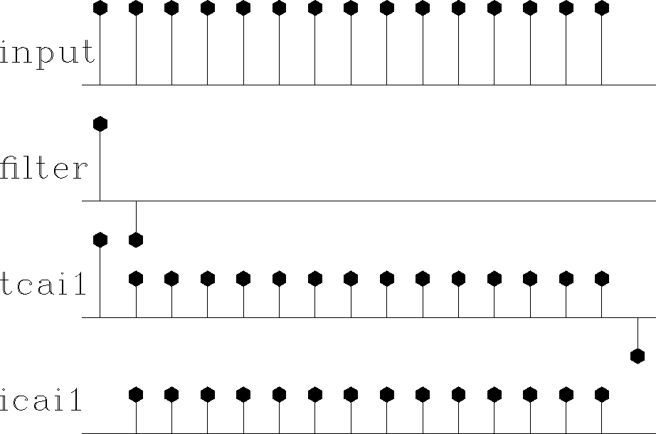
The
end effects
of the convolution modules are summarized
in Figure ![[*]](http://sepwww.stanford.edu/latex2html/cross_ref_motif.gif) .
.
conv90
Figure 2
Example of convolution end-effects.
From top to bottom:
input;
filter;
output of tcai1();
output of icaf1() also with (lag=1).
|
|  |


Next: Zero padding is the
Up: FAMILIAR OPERATORS
Previous: Transient convolution
Stanford Exploration Project
4/27/2004
![\begin{displaymath}
\left[
\begin{array}
{c}
y_3 \\
y_4 \\
y_5 \\
y_6...
...
\begin{array}
{c}
b_1 \\
b_2 \\
b_3 \end{array} \right]\end{displaymath}](img32.gif)
![\begin{displaymath}
\left[
\begin{array}
{c}
y_3 \\
y_4 \\
y_5 \\
y_6...
...
\begin{array}
{c}
b_1 \\
b_2 \\
b_3 \end{array} \right]\end{displaymath}](img32.gif)
![\begin{displaymath}
\left[
\begin{array}
{c}
\hat b_1 \\
\hat b_2 \\
\hat b...
...y}
{c}
y_3 \\
y_4 \\
y_5 \\
y_6
\end{array} \right]\end{displaymath}](img33.gif)
![\begin{displaymath}
\left[
\begin{array}
{c}
y_1 \\
y_2 \\
y_3 \\
y_4...
...
\begin{array}
{c}
b_1 \\
b_2 \\
b_3 \end{array} \right]\end{displaymath}](img34.gif)
![[*]](http://sepwww.stanford.edu/latex2html/cross_ref_motif.gif) .
.