Geoestimation: empty bin example

The basic formulation of a geophysical estimation problem consists of setting up two goals, one for data fitting, and the other for model smoothing. We have data $\bold d$,a map or model $\bold m$,a transformation and a roughening filter $\bold A$,like the gradient $\nabla$ or the helix derivative $\bold H$.The two goals may be written as:

$$\begin{eqnarray} \bold 0 &\approx& \bold r \quad = \quad\bold L \bold m - \bold d \\ \bold 0 &\approx& \bold p \quad = \quad\bold A \bold m\end{eqnarray}$$ (12) (13)

which defines two residuals, a data residual $\bold r$,and a model residual $\bold p$, which are usually minimized by iterative conjugate-gradient, least-squares methods. A common case is ``minimum wiggliness'' when $\bold A$ is taken to be the gradient operator. The gradient is not invertable so we cannot precondition with its inverse. On the other hand, since $-\nabla^2 = \bf div \cdot grad = H'H$,taking $\bold A$ to be the helix derivative $\bold H$,we can invert $\bold A$ and proceed with the preconditioning: We change the free variable in the fitting goals from $\bold m$ to $\bold p$(by inverting (13)) with $\bold m = \bold A^{-1} \bold p$and substituting into both goals getting new goals

$$\begin{eqnarray} \bold 0 &\approx& \bold L \bold A^{-1} \bold p - \bold d \\ \bold 0 &\approx& \bold p\end{eqnarray}$$ (14) (15)

In my experience, iterative solvers find convergence much more quickly when the free variable is the roughened map $\bold p$rather than the map $\bold m$ itself.

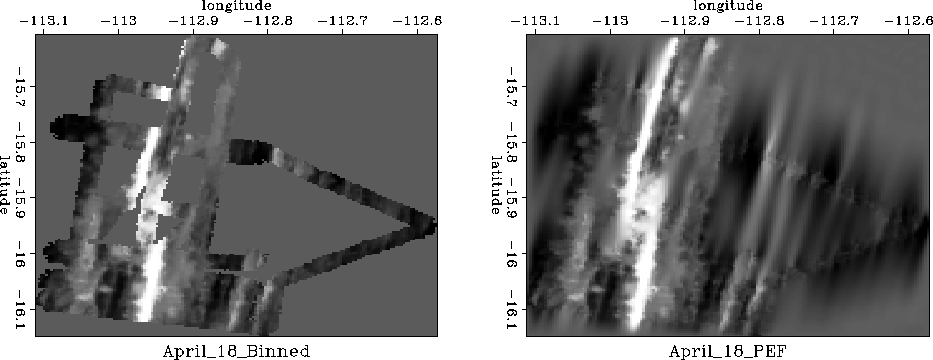
Figure 11 (left) shows ocean depth measured by a Seabeam apparatus.

 

seapef
Figure 11 Filling empty bins with a prediction-error filter.

Locations not surveyed are evident as the homogeneous gray area. Using a process akin to ``blind deconvolution'' a 2-D prediction error filter $\bold A$ is found. Then missing data values are estimated and shown on the right. Preconditioning with the helix speeded this estimation by a factor of about 30. The figure required a few seconds of calculation for about 10⁵ unknowns.