Matrix view of the helix

Finally, let us look at the helix from the view of matrices and numerical analysis. This is not easy because the matrices are so large. Discretize the (x,y)-plane to an $N\times M$ array and pack the array into a vector of $N\times M$ components. Likewise pack the Laplacian operator $\partial_{xx}+\partial_{yy}$into a matrix. For a $4\times 3$ plane, that matrix is shown in equation (8).  

$$-\ \nabla^2 \quad = \quad \begin{array} {\vert rrrr\vert rrr... ...& \cdot & \cdot & -1 & 4 \\ &&&& &&&& &&& \\ \hline\end{array}$$ (8)

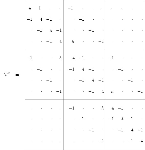
The two-dimensional matrix of coefficients for the Laplacian operator is shown in (8), where, on a Cartesian space, h=0, and in the helix geometry, h=-1. (A similar partitioned matrix arises from packing a cylindrical surface into a $4\times 3$ array.) Notice that the partitioning becomes transparent for the helix, h=-1. With the partitioning thus invisible, the matrix simply represents one-dimensional convolution and we have an alternative analytical approach, one-dimensional Fourier Transform. We often need to solve sets of simultaneous equations with a matrix similar to (8). The method we use is triangular factorization.

Although the autocorrelation $\bold r$ has mostly zero values, the factored autocorrelation $\bold h$ from (5) has a great number of nonzero terms, but fortunately they seem to be converging rapidly (in the middle) so truncation (of the middle coefficients) seems reasonable. I wish I could show you a larger matrix, but all I can do is to pack the signal $\bold h$ into shifted columns of a lower triangular matrix $\bold H$ like this:  

$$\bold H \ = \ \ \left[ \begin{array} {rrrrrrrrrrrr} 1.8&\cd... ...ot&\cdot&\cdot&\cdot& -.6& -.2& 0.0& -.6& 1.8\end{array}\right]$$ (9)

If you will allow me some truncation approximations, I now claim that the laplacian represented by the matrix in equation (8) is factored into two parts $-\nabla^2 =\bold H'\bold H$which are upper and lower triangular matrices whose product forms the autocorrelation seen in (8). Recall that triangular matrices allow quick solutions of simultaneous equations by backsubstitution. That is what we do with our deconvolution program.