Inversion to Zero Offset Canadian Data Example
(courtesy of Pan Canadian Petroleum)
An original data set that was considered oversampled and
was decimated in order to simulate a more economic acquisition
geometry.
Acquisition Geometry
The geometry of the processed data (after decimation and
after removal of all traces with suspected signal to noise ratio)
is shown in figures 1 and 2.
The geometry is mostly cross-spread, except two receiver lines which
run in parallel to the shot lines. These two receiver lines cause
some fold anomalies.
The offset standard deviation is relevant to the footprint of the
suppression of low-velocity multiples by stacking.

Fig 1. Map of shot and receiver points
(a) 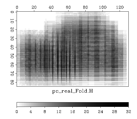
(b) 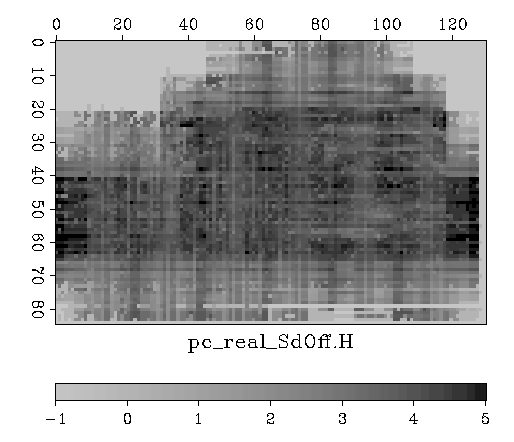
Fig2. Maps of (a) midpoint fold and (b) offset standard deviation
Bull's Eyes Analysis
Bull's Eyes analysis is shown in Figure 3.
This analysis indicates that Calibrated DMO is needed to equalize
the coverage. With IZO, it is expected that sub-binning to 17.5m
(half the nominal bin size) will provide better resolution.
(a) 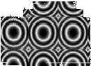 (b)
(b) 
(c) 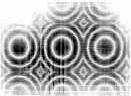 (d)
(d) 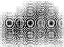
(e) 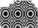 (f)
(f) 
(g)  (h)
(h) 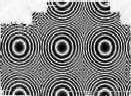
(i) 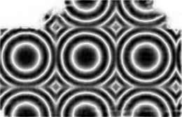 (j)
(j) 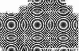
Fig. 3:
(a) NMO, 35m bins, 20 Hz. (b) NMO, 35m bins, 50 Hz.
(c) DMO, 35m bins, 20 Hz. (d) DMO, 35m bins, 50 Hz.
(e) Calibrated DMO, 35m bins, 20 Hz. (f) Calibrated DMO, 35m bins, 50 Hz.
(g) IZO, 35m bins, 20 Hz. (h) IZO, 35m bins, 50 Hz.
(i) IZO, 17.5 bins, 20 Hz. (j) IZO, 17.5 bins, 50 Hz.
Results
The data were first processed with conventional
deconvolution velocity analysis,
surface consistent statics, and normal moveout.
To improve the signal to noise ratio,
all traces suspected of having low signal to noise ratio were removed.
Also, all traces were balanced by the amplitude of the 98th quantile,
and clipping all values above 1 after this trace balance.
(The 98th quantile is a value which is larger than 98% of the data
and smaller than 2% of the data.)
Following the signal to noise enhancing processing the data were imaged using
Calibrated DMO and IZO.

Fig 4: Cube after Calibrated DMO on the left.
Cube after IZO on the right.
Each cube is views through a time slice, and two normal cross-sections.
The thin black lines indicate the locations of the slices and the sections.
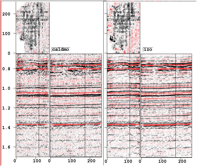
Fig. 5:
Other slices and sections through the same cubes of Fig 4.
The alternative slices are shown because the time slices in
Fig 5 is taken on a multiple and shows a footprint which is related
to the map of offset standard deviation on Fig 2b.
(a) 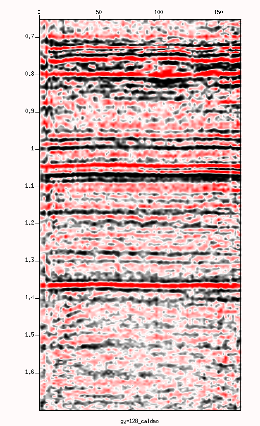
(b) 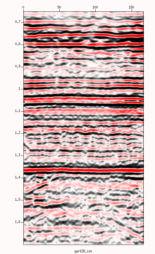
Fig 6: Cross line section at y=128.
(a) Calibrated DMO processing. (b) IZO.
Note the dipping reflectors at 1.4 to 1.6 seconds.
(a) 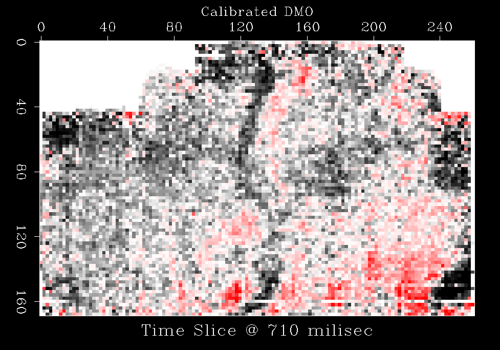
(b) 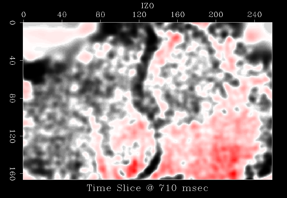
Fig 7: Time slice at 710 msec.
(a) Calibrated DMO processing. (b) IZO.
Note the effect of the half-binning to 17.5 meters on the IZO image.