Next: A first reservoir flow
Up: Reservoir fluid flow simulator
Previous: Reservoir fluid flow simulator
The finite difference reservoir flow simulator for a single phase
is a straightforward explicit finite difference implementation of
the corresponding fluid flow equation 8:
![\begin{displaymath}
u_{t+1}^{x,y} - u_t^{x,y} =
\hat{d} [(u_t^{x-1,y} -2 u_t^{x,y} + u_t^{x+1,y})
+ (u_t^{x,y-1} -2 u_t^{x,y} + u_t^{x,y+1})] \end{displaymath}](img26.gif)
where  is the transmissibility.
Each grid point represents a homogeneous subsurface cell.
A straightforward stability analysis
(see the finite difference wave equation section)
yields
is the transmissibility.
Each grid point represents a homogeneous subsurface cell.
A straightforward stability analysis
(see the finite difference wave equation section)
yields  and
and  .
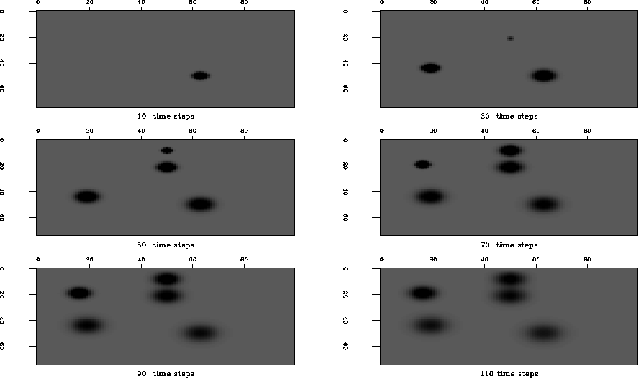
Figure 1 shows snapshots of a reservoir of constant
transmissibility and random sources of pressure. The pressure
impulses diffuse over time as we would expect from a solution
to a parabolic differential equation.
impFlowSnap
.
Figure 1 shows snapshots of a reservoir of constant
transmissibility and random sources of pressure. The pressure
impulses diffuse over time as we would expect from a solution
to a parabolic differential equation.
impFlowSnap
Figure 1
Snapshots of the reservoir fluid flow simulator for a medium of
constant transmissibility and randomly located point sources of pressure.
The panels show the pressure field as time increases from left to
right and top to bottom. An impulsive source generates an impulse that
diffuses over time.


Next: A first reservoir flow
Up: Reservoir fluid flow simulator
Previous: Reservoir fluid flow simulator
Stanford Exploration Project
3/9/1999