AVO THEORY IN ACOUSTIC AND ELASTIC MEDIA

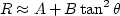
Under the assumption of small incident angle, there is a well-known linearized Zoeppritz equation (). Because we only consider the incident angle less than 35 degree, we have omitted the C term in the original form. For the acoustic and elastic media, the expressions for the reflection coefficients are different. Acoustic AVO approximation

$$R \approx A + B\tan^2{\theta}$$ (189)

where

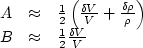$$\begin{array} {lll} A & \approx & \frac{1}{2} \left (\frac{... ...\\ B & \approx & \frac{1}{2} \frac{\delta V}{V} \\ \end{array}$$ (190)

Elastic AVO approximation

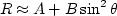$$R \approx A + B\sin^2{\theta}$$ (191)

where

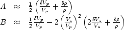$$\begin{array} {lll} A & \approx & \frac{1}{2} \left (\frac{... ... V_s}{V_s} + \frac{\delta \rho}{\rho} \right ) \\ \end{array}$$ (192)

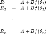
Using the reflection coefficient R and specular incident angle $\theta$, we find the solution for intercept and slope is a least-squares problem.

$$\begin{array} {lll} R_1 & = & A + B f(\theta_1) \\ R_2 & =... ... & \\ & \cdot & \\ R_n & = & A + B f(\theta_n) \\ \end{array}$$ (193)

The resulting estimates of A and B are given by

$$\left[ \begin{array} {c} A \\ B \end{array}\right ] = \lef... ...{i}^{N} R_i \\ \sum_{i}^{N} R_i f(\theta_i)\end{array}\right ]$$ (194)

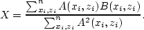
Getting AVO intercept and slope is not our final goal. The purpose of AVO analysis is to display the V_p/V_s anomaly in the subsurface. This anomaly is a very important hydrocarbon indication, especially for gas-charged reservoirs. Here we use the fluid-line technique to highlight this anomaly. Assume there is a linear relation

A X + B = 0 (195)

between intercept A and slope B. We specify a window with reasonable size and use least squares algorithm to estimate the coefficient X. Similar to $\cos{\theta}$, we get an expression for X

$$X = \frac{\sum_{x_i,z_i}^{n} A(x_i,z_i)B(x_i,z_i)} {\sum_{x_i,z_i}^{n}A^2(x_i,z_i)}.$$ (196)

The A X + B section is called the fluid-line section, which highlights the V_p/V_s anomaly.