Tetragonal eikonal equation

In the 3-D Cartesian coordinates, the eikonal equation is expressed as  

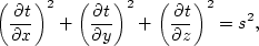$$\left (\frac{\partial t}{\partial x} \right )^2+ \left (\fra... ...ght )^2+ \left (\frac{\partial t}{\partial z} \right )^2 = s^2,$$ (152)

where t stands for traveltime and s for slowness. The 2-D counterpart is given by omitting one term from the above equation.  

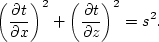$$\left (\frac{\partial t}{\partial x} \right )^2+ \left (\frac{\partial t}{\partial z} \right )^2 = s^2.$$ (153)

The Cartesian expressions have no crossing terms because of the orthogonality. If we define a tetragonal coordinate which has a transform relation () with the Cartesian coordinates as shown in Figure  

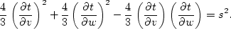
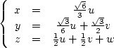$$\left\{ \begin{array} {ccc} x & = & \frac{\sqrt{6}}{3}u \\ ... ... z & = & \frac{1}{2}u + \frac{1}{2}v + w \end{array} \right .$$ (154)

 

coord Figure 1 The tetragonal coordinates used in this paper. It reduces to the trigonal coordinates by omitting axis u.

and then substitute equation () into () and (), we can get the following eikonal equation in the tetragonal (3-D) and trigonal (2-D) coordinates.

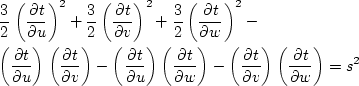$$\begin{eqnarray} &&\frac{3}{2} \left (\frac{\partial t}{\partial u} \right )^2+ ... ...tial v} \right ) \left (\frac{\partial t}{\partial w} \right )=s^2\end{eqnarray}$$ (155)

$$\frac{4}{3} \left (\frac{\partial t}{\partial v} \right )^2+... ... v} \right ) \left (\frac{\partial t}{\partial w} \right )=s^2.$$ (156)

The fast-marching algorithm is an upwind first-order discretization of the above eikonal equation. In next section, we show that it reduces to solving a quadratic equation. The key feature of this algorithm is a carefully selected order of traveltime evaluation. In the Cartesian coordinates, each point with known traveltime can update four equally-spaced neighboring points in 2-D and six in 3-D, as shown in Figure and . In the trigonal and tetragonal coordinates, these two numbers are six and twelve respectively, as shown in Figure and . Since the fast-marching eikonal solver is based on the plane wave assumption, more equally-spaced neighboring points mean a better approximation to the assumption. Therefore, TFMES should be more accurate than its Cartesian counterpart.

 

cart2D Figure 2 2-D updating scheme in the Cartesian coordinates. Traveltime at point (i,j) is known and four equally-spaced neighboring points' traveltimes are candidates for updating.

 

cart3D Figure 3 3-D updating scheme in the Cartesian coordinates. Traveltime at point (i,j,k) is known and six equally-spaced neighboring points' traveltimes are candidates for updating.

 

nonorth2D Figure 4 2-D updating scheme in the trigonal coordinates. Traveltime at point (i,j) is known and six equally-spaced neighboring points' traveltimes are candidates for updating.

 

nonorth3D Figure 5 3-D updating scheme in the nonorthogonal coordinates. Traveltime at point (i,j,k) is known and twelve equally-spaced neighboring points' traveltimes are candidates for updating.

Alkhalifah and Fomel have shown that the fast-marching algorithm in the polar coordinates is also more accurate than the Cartesian implementation. The reason is that the circular (2-D) or spherical (3-D) axis in the polar coordinates closely matches the wavefront when the media are relatively smooth. However, the polar implementation needs to transform the velocity model from the Cartesian to the polar coordinates for each single source, which makes it inconvenient. The grid size in the polar coordinates becomes larger and larger with the increase of radius. Therefore, some of the detailed velocity variation can be missed easily. Free of these problems, TFMES is more flexible and efficient than the polar implementation.