2: Warping $\bold H_i^{\prime}(x,y)$ to match the well logs

Qualitatively, we can express the desired attributes of the output model $\tilde{\bold H}_i(x,y)$:

1.

At the well locations, the difference between $\tilde{\bold H}_i(x,y)$and the well log data should vanish.

2.

At distances far from any well, the output model should match (in a least squares sense) $\bold H_1^{\prime}(x,y)$ and $\bold H_2^{\prime}(x,y)$ as closely as possible - in magnitude and also in relative shape.

This is sound logic; the well log data is (for the sake of simplicity) assumed to be perfectly accurate, so at the well locations, the output model is rigidly constrained to match these measurements. On the other hand, when we are far from any well location, the only source of information is $\bold H_i^{\prime}(x,y)$.

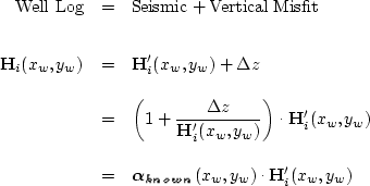
This method is strictly a vertical correction. It is naïve to assume that the misfit between the seismic horizon and the well logs is purely vertical, but well log measurements place no direct horizontal constraints on the output model. However, in the ``Future Work'' section I discuss how simple anisotropy can manifest itself in seismic data through vertical misfit, and how, through a simple inversion scheme, we may be able to quantify the degree of anisotropy.

We can directly measure the vertical discrepancy between $\bold H(x,y)$ and $\bold H_i^{\prime}(x,y)$ at the well locations, (x_w,y_w):

$$\begin{eqnarray} \mbox{Well Log} &=& \mbox{Seismic} + \mbox{Vertical Misfit} \no... ...math$\alpha_{known}$}(x_w,y_w) \cdot \bold H_i^{\prime}(x_w,y_w) \end{eqnarray}$$ (105)

Now solve a missing data problem to obtain a smooth 2-D function $\alpha$(x,y), whose value is already known at the well locations ($\alpha_{known}$(x,y)).

$$\begin{eqnarray} \bold J_{well}(\mbox{\boldmath$\alpha - \alpha_{known}$}) &\app... ...dmath$\epsilon$}\, \nabla^2 \mbox{\boldmath$\alpha$} &\approx& 0 \end{eqnarray}$$ (106) (107)

$\bold J_{well}$ is the ``well location selector'' operator, similar to $\bold J_{seis}$ in Equation (). I choose the 2-D Laplacian, $\bf \nabla^2$, as the regularization operator, because the vertical misfit is in general not dependent on the geology of the horizon which we're trying to update. Therefore we opt for the isotropic smoothing qualities of $\bf \nabla^2$, rather than those of a PEF. However, as a future project I suggest implementing this methodology in a recursive layer-stripping scheme. In this case, making the regularization operator dependent on the geometrical and physical properties of the overlying horizons makes sense, though the details have not yet been formalized.

This problem is grossly underdetermined ($\approx$ 15 known values vs. 1600 points in model space), so even for a good choice of ${\epsilon}$, convergence is slow - too slow, in fact, to make this method practical for application to real-world problems. To solve this problem, I use preconditioning, defined as any change of variables which speeds convergence of an iterative scheme.

In general, the preconditioning operator $\bf S$ is defined by  

$$\bf m = Sp$$ (108)

where ${\bf m}$ is the model variable and $\bf p$ is the so-called ``preconditioned variable.'' The choice of $\bf S$ is arbitrary. However, () proposes a simple, yet highly effective choice for $\bf S$: the inverse of the regularization operator. Our regularization operator ($\nabla^2$) is 2-D convolution, so its inverse is obtained by 2-D deconvolution - in general an ill-defined process. But the Helix Transform () comes to the rescue, allowing us to use the simple 1-D algorithm to perform 2-D deconvolution.

First wrap $\bf \nabla^2$ onto a helix, then unroll it to create a long 1-D filter, as shown in Figure . Through the process of spectral factorization, we compute a minimum phase filter $\bf a$ whose autocorrelation is $\bf \nabla^2$: $\bf a^{\prime} a = \nabla^2$. Since $\bf a$ is minimum phase, successive convolution with $\bf a$ and $\bf a^{\prime}$ is multiplication with lower and upper diagonal matrices, respectively. Therefore, the inverse operation, deconvolution, is matrix inversion: $\bf (\nabla^2)^{-1} = (a^{\prime} a)^{-1} = a^{-1} (a^{\prime})^{-1}$, which can be done very quickly in this case with simple backsubstitution, an ${\cal O}(n)$ operation! For more details on the spectral factorization methods used at SEP, see (), or more recently, ().

 

helix
Figure 4 Schematic of the helical representation of $\nabla^2$. Adapted from a Mathematica drawing by Sergey Fomel.

Now that we can compute the preconditioner $\bf (\nabla^2)^{-1}$ with confidence, repose the original problem. First apply the following change of variables:  

$$\bf \alpha = (\nabla^2)^{-1} p$$ (109)

Substitute Equation () into Equations () and () to obtain

$$\begin{eqnarray} \bf J_{well}((\nabla^2)^{-1} p - \mbox{\boldmath$\alpha_{known}$}) &\approx& 0 \nonumber\\ \bf \epsilon p &\approx& 0 \end{eqnarray}$$ (110)

We solve for $\bf p$ iteratively, then convert back to $\alpha$ via equation . Figure shows the resultant $\alpha$(x,y) for both the shallow and deep horizons. Does preconditioning work? Yes! In this example, the rate of convergence is increased by two orders of magnitude by preconditioning, e.g., roughly 1000 versus 10 CD iterations.

 

alpha-both
Figure 5 Seismic warp functions $\boldmath\alpha(x,y)$, for the shallow and deep horizons.

Now we compute the final output model, $\bf \tilde{H}_i(x,y)$  

$$\bf \tilde{H}_i(x,y) = {\bold H}^{\prime}_i(x,y) \cdot \mbox{\boldmath$\alpha(x,y)$}$$ (111)

The results for both shallow and deep horizons are shown in figures and , respectively.

 

wellmap-2000
Figure 6 Final result: updated shallow horizon.

 

wellmap-2300
Figure 7 Final result: updated deep horizon.