The model

The original Marmousi model was built to resemble an overall continental drift geological setting. Numerous large normal faults were created as a result of this drift. The geometry of Marmousi is based somewhat on a profile through the North Quenguela through the Cuanza basin Versteeg (1993). The target zone is a reservoir located at a depth of about 2500 m. The model contains many reflectors, steep dips, and strong velocity variations in both the lateral and the vertical direction (with a minimum velocity of 1500 m/s and a maximum of 5500 m/s). However, there is no clear evidence of the Marmousi model intended sediment or rock distribution, and this includes the distribution of shales. As a result, the same discard for sediment distribution, that went into building the sediment content of the original model, is used here. This is justified by the fact that our goal is purely imaging. Nobody seemed to care for the geological aspect of the model.

 

veleta
Figure 1 Top: The original Marmousi velocity model given by IFP. Bottom: An $\eta$ model built using the above Marmousi velocity model and constraining the horizontal velocity to increase linearly. The values of $\eta$ range from zero to 0.274. The vertical P-wave velocity for this VTI model is taken to equal v, shown on top.

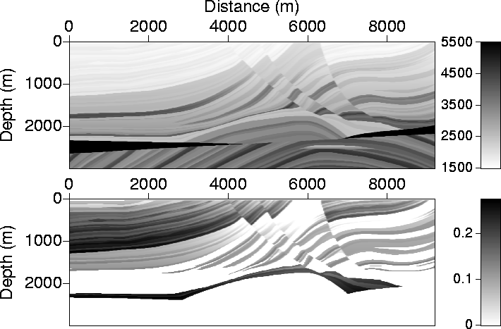Figure 1 (top) shows the original velocity model used by the Institute Francaise du Petrole (IFP) to generate the Marmousi synthetic data set. Figure 1 (bottom) shows an $\eta$ model that is based on the following two hypothetical assumptions:

• Anisotropy increases as velocity decreases (shales have low velocity overall).
• The horizontal velocity gradually increases with depth.

The second assumption means that although the NMO velocity may vary erratically, the horizontal velocity retains a relatively linear increase with depth. Although there is no settled proof that the above assumptions are accurate representation of the subsurface behavior in the presence of anisotropy, my personal experience suggests that they are at least plausible. Nevertheless, my goal is not to build a realistic geological model, but rather to obtain anisotropic data from a complex model that we can use to test existing anisotropic algorithms.

As mentioned in the previous section, three parameters describe wave propagation in an acoustic VTI model. The parameter $\eta$ is perhaps the most influential with respect to the anisotropic influence on imaging and focusing Alkhalifah and Tsvankin (1995). On the other hand, v_v is responsible for the depth positioning of reflectors. In this model, v_v is set to equal the NMO velocity, v, because theoretically v_v is unresolvable from surface P-wave seismic data Alkhalifah et al. (1997); Alkhalifah (1997c). It can only be obtained from well data, and such information is beyond the scope of this paper. Apart from the imaging issue, fitting an isotropic model to anisotropic data results in over-estimation of NMO velocity, and thus over-estimation of depth even if the vertical velocity equals the NMO velocity Alkhalifah (1997b).

For the VTI model, the NMO velocity, v, is given by the IFP original velocity model. The anisotropy parameter $\eta$ is built to inherent the layering of the original IFP velocity model. This task is accomplished by imposing three guidelines on $\eta$:

• $\eta$=0 for layers with v=1500 m/s, which corresponds to the water layer.
• $\eta$=0 for layers with v>2500 m/s, which are velocities higher than those of a typical shale layer.
• $\eta$ satisfies equation (1) and v_h=1750+0.8 z m/s in all other layers of the model.

As a result, interval $\eta$, shown in the bottom panel of Figure 1 ranges from zero to 0.274, which is a practical range for $\eta$ in the subsurface Alkhalifah (1997a,b). Specifically, $\eta$=0.274 corresponds to a difference between the horizontal to vertical P-wave velocity of about 25 percent, which is a reasonable value Banik (1984); Harris et al. (1994). Meanwhile, effective $\eta$ Alkhalifah (1997b), which represents an average of the overburden $\eta$ influence, has overall lower values than the interval $\eta$. It is the effective $\eta$, not the interval $\eta$, that has a direct impact on imaging.