|
deepBottom
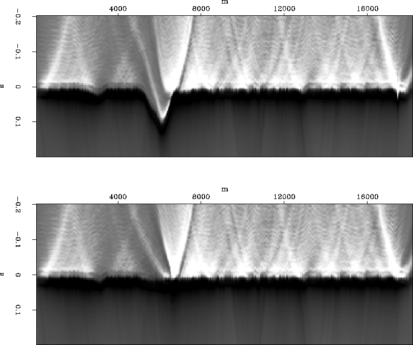
Figure 1 Downward continuing correlations to the calculated sea floor depth shows some depth error where there is large topography (top). Adding a residual depth term corrects the errors (bottom). |  |
The multiple suppression algorithm applied here is that formulated by Berryhill Berryhill and Kim (1986). It is similar in principle to just shifting the data by a lag equal to one multiple period and subtracting, except that a more sophisticated operator is used. Kirchoff datuming is employed to model an additional bounce from the surface to the seafloor and back, so that the original primary and multiple energy, P + M1 + M2 + ..., emulates strictly multiples, M1' + M2' + M3' + ....
The continuation velocity is known (water), though the seafloor does need to be picked. Here I pick one seafloor point, and do correlation in a sliding window around the seafloor. I then migrate the correlations with water velocity, pick the max in each trace as the seafloor, and calculate depth.
As a test, the correlations can be downward continued to the water bottom. Ideally they should wind up at zero time, but there is noticeable misfit in the deep water data, where there is strong seafloor topography, despite the initial migration, as shown in the top of Figure 1. I calculate a residual depth correction by estimating statics on the misfit, add it to the original depth estimate and downward continue again. The bottom of Figure 1 shows the correlations downward continued to the revised seafloor.
|
deepBottom
Figure 1 Downward continuing correlations to the calculated sea floor depth shows some depth error where there is large topography (top). Adding a residual depth term corrects the errors (bottom). |  |
Once the data are upward continued, the original and redatumed data are subtracted with the hope that
| P + (M1 - M1') + (M2 - M2') + ... = P | (1) |
| |
(2) |