


Next: synthetic test
Up: Ordinary differential equation representation:
Previous: Ordinary differential equation representation:
The kinematic  -continuation equation (19) corresponds
to the following linear fourth-order dynamic equation
-continuation equation (19) corresponds
to the following linear fourth-order dynamic equation
| 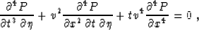 |
(21) |
where the t coordinate refers to the vertical traveltime  , and
, and
 is the migrated image, parameterized in the anisotropy
parameter . To find the correspondence between equations
(19) and (21), it is sufficient to apply a
ray-theoretical model of the image
is the migrated image, parameterized in the anisotropy
parameter . To find the correspondence between equations
(19) and (21), it is sufficient to apply a
ray-theoretical model of the image
|  |
(22) |
as a trial solution to (21). Here the surface  is the anisotropy continuation ``wavefront'' - the image of a
reflector for the corresponding value of , and the function A
is the amplitude. Substituting the trial solution into the partial
differential equation (21) and considering only the terms
with the highest asymptotic order (those containing the fourth-order
derivative of the wavelet f), we arrive at the kinematic equation
(19). The next asymptotic order (the third-order derivatives
of f) gives us the linear partial differential equation of the
amplitude transport, as follows:
is the anisotropy continuation ``wavefront'' - the image of a
reflector for the corresponding value of , and the function A
is the amplitude. Substituting the trial solution into the partial
differential equation (21) and considering only the terms
with the highest asymptotic order (those containing the fourth-order
derivative of the wavelet f), we arrive at the kinematic equation
(19). The next asymptotic order (the third-order derivatives
of f) gives us the linear partial differential equation of the
amplitude transport, as follows:
|  |
(23) |
We can see that when the reflector is flat ( and
and
 ), equation (23) reduces to the equality

and the amplitude remains unchanged for different . This is of
course a reasonable behavior in the case of a flat reflector. It
doesn't guarantee though that the amplitudes, defined by
(23), behave equally well for dipping and curved
reflectors. The amplitude behavior may be altered by adding low-order
terms to equation (21). According to the ray theory, such
terms can influence the amplitude behavior, but do not change the
kinematics of the wave propagation.
An appropriate initial-value condition for equation (21) is
the result of isotropic migration that corresponds to the  section in the
  domain. In practice, the initial-value
problem can be solved by a finite-difference technique.
domain. In practice, the initial-value
problem can be solved by a finite-difference technique.
Next: synthetic test
Up: Ordinary differential equation representation:
Previous: Ordinary differential equation representation:
Stanford Exploration Project
11/11/1997