Better stationary-phase approximations

Although previous approximations of p_h for horizontal reflectors in VTI media (Appendix B) yield adequate results, better approximations based on perturbation theory can further enhance the accuracy of the migration. The theory is based on expressing the solution in terms of power-series expansions of parameters that are expected to be small. As a result, higher power terms have smaller contributions, and as a result, they are usually dropped. The degree of truncation depends on the convergence behavior of the series. I will apply the perturbation theory to evaluate the stationary-phase solution at p_x=0 and p_x=p_h in VTI media.

In the case of p_x=0, the stationary point solution p_h, as we saw earlier, satisfies  

$$8 \eta^3 X^2 (1+2 \eta) y^4 - 4 \eta^2 X^2 (3+8 \eta) y^3 + ... ...X^2 (1+4 \eta) y^2 - [X^2 (1+8 \eta)+ \tau^2 v^2] y + X^2 = 0,$$ (42)

where y=p_h² v². Analytical solutions for this quartic equation in y exist. They are, however, complicated, and some of them actually do not exist ($\rightarrow \infty$) for $\eta$=0. Recognizing that both $\eta$ and p_h can be small, we can drop terms beyond the quadratic, as done in Appendix B, and solve the resultant quadratic equation analytically. We can also benefit from fact that $\eta$ can be small and use perturbation series, that is, apply a power-series expansion in terms of $\eta$. Unlike weak anisotropy approximations, the resultant solution yields good results even for strong anisotropy ($\eta\gt.5$). The key here is to recognize the behavior of the series for large powers of $\eta$ using Shanks transforms. According to the perturbation theory (Bender and Orszag, 1978), the solution of equation (C-1) can be represented in a power-series expansion in terms of $\eta$as follows  

$$y = \sum_{i=0}^{\infty} {y_i \eta^i},$$ (43)

where y_i are coefficients of this power series. For practical applications, the power series of equation (C-2) is truncated to n terms as follows  

$$A_n = \sum_{i=0}^{n} {y_i \eta^i}.$$ (44)

The coefficients, y_i, are determined by inserting the truncated form of equation (C-2) (three terms of the series are enough here) into equation (C-1) and then solving for y_i, recursively. Because $\eta$ is a variable, we can set the coefficients of each power of $\eta$ separately to equal zero. This gives a sequence of equations for the y_i expansion coefficients. For example, y₀ is obtained directly from setting $\eta$=0, and the result corresponds to the solution for isotropic media. For large $\eta$, A_n converges slowly to the exact solution, and, therefore, yields sub-accurate results when used, even if we go up to A₁₀. Truncating after the second term (linear in $\eta$, A₁) is referred to as the weak anisotropy approximation. Using Shank transforms (Bender and Orszag, 1978), one can predict the behavior of the series for large n, and, therefore, eliminate the most pronounced transient behavior of the series (to eliminate the term that has the slowest decay). Following Shanks transform, the solution is evaluated using the following relation

$$y_s = \frac{A_2 A_0 - A_1^2}{A_2+A_0-2 A_1}.$$

After some tedious algebra, done using primarily the Mathematica program, p_h corresponding to horizontal events is given by  

$$p_{h0} = \frac{1}{v} {\sqrt{{\frac{{X^2}\,\left( {X^6} - 6... ...a \right) \,{{\tau }^4} + 4\,{v^6}\,{{\tau }^6} \right) }}}}.$$ (45)

Unlike equation (B-12), which corresponds to the solution of the quadratic truncation of equation (C-1), equation (C-4) is valid for all practical models. No validity conditions are required here.

The same steps used above to evaluate p_h for p_x=0 is used for the case p_x=p_h (p_s=0), and, as a result,  

$$p_{hs} = \frac{1}{v} {\sqrt{{\frac{{X^2}\,\left( 16\,{X^6} -... ...\eta \right) \,{{\tau }^4} + {v^6}\,{{\tau }^6} \right) }}}}.$$ (46)

Now, we insert the new definitions of p_h0 and p_hs into equation (B-17):  

$$p_h = p_{h0} \frac{(1-2 \eta p_x^2 v^2)^4 (\frac{1-p_x^2 v^... ... \eta p_x^2 v^2-6 \eta (1+2 \eta) p_x^4 v^4]} [a(p_{h0})p_x+1],$$ (47)

where

$$a= \frac{1}{p_{h0}} \frac{1+4 \eta p_x^2 v^2-6 \eta (1+2 \et... ...eta p_x^2 v^2}{ 1-2 \eta p_x^2 v^2})^{3/2}}-\frac{1}{p_{hs}}.$$

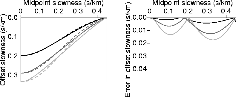
Figure C-1 shows a comparison between the exact p_h solution of equation (B-1) (obtained numerically) and that given by equation (C-6) as a function of p_x for three sets of $\frac{X}{\tau}$. The absolute difference between the two solutions is also displayed. Clearly, results, obtained using the modified equation, are far superior to the ones obtained in Appendix B for VTI media.

 

ph3sheta2m
Figure 23 Left: Values of p_h as a function of p_x calculated numerically (solid curves), and calculated analytically (dashed curves) using equation (C-6). Right: The absolute difference between the two curves on the left. The medium is homogeneous and isotropic with v=2.0 km/s. The black curve corresponds to $\frac{X}{\tau}$=1.0 km/s, the dark-gray curve corresponds to $\frac{X}{\tau}$=2.0 km/s, and the light gray curve corresponds to $\frac{X}{\tau}$=3.0 km/s.