


|
OffAzsm
Figure 4 Offset-azimuth distribution of the test data set. The vertical bars show the boundaries among the offset ranges that were used for partial stacking. | 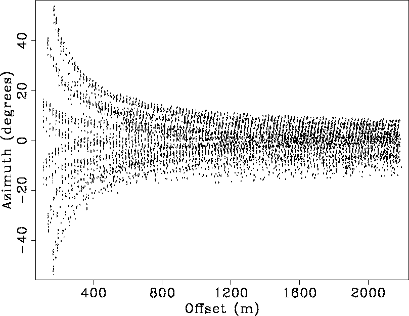 |


I tested the common-azimuth imaging procedure on a data set recorded in the North Sea. The data require 3-D prestack depth migration to be properly imaged because of a shallow chalk layer with variable thickness, and a deeper salt layer with a central upswelling Hanson and Witney (1995). The same data set was used to test separately the two main components of the common-azimuth imaging procedure: AMO Biondi et al. (1996b) and common-azimuth migration Biondi (1996).
The data-acquisition configuration was dual-source and triple streamer. The nominal common-midpoint spacing was 9.375 m in the in-line direction, and 25 m in the cross-line direction. The cable length was 2,200 m, with maximum feathering of approximately 17 degrees. Figure 4 shows the offset-azimuth distribution of a small subset of the data traces. As it is typical for such acquisition geometry, the figure shows six distinct trends, which are most distinguishable at small offsets; each trend corresponding to individual source-streamer pairs.
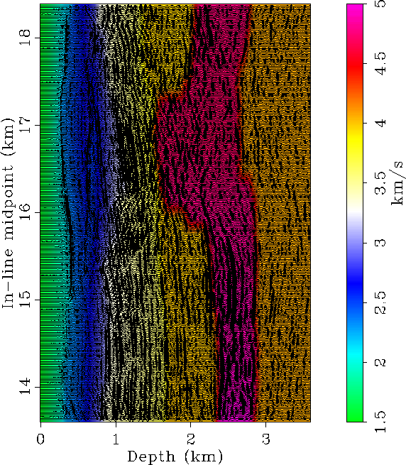
Figure 5 demonstrates the effectiveness of the common-azimuth imaging procedure to image 3-D data in the presence of a complex velocity function. The figure shows an in-line section extracted from a migrated cube imaged by common-azimuth migration. The superposition of the migrated results onto the velocity model shows that common-azimuth migration successfully imaged the reflectors and correctly positioned them in depth. The migrated salt boundaries overlap quite precisely with the salt boundaries identified by the sharp variations in the velocity model. The target reflectors below the salt layer are also well imaged, though it seems that their focusing could be improved by further refinements of the velocity function.
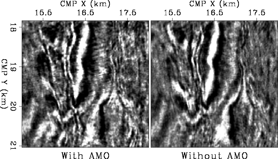
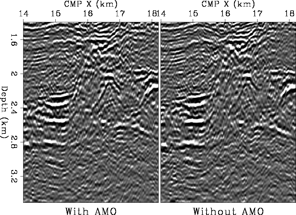
Figure 6 and Figure 7 demonstrate the advantages of including AMO into the common-azimuth imaging procedure. The figures show sections extracted from image cubes obtained by common-azimuth migration. The sections on the left were obtained including AMO in the processing sequence; the ones on the right by transforming the data to common-azimuth using residual NMO followed by midpoint interpolation. To make the comparison as fair as possible to the conventional method of simple NMO-stacking, its accuracy was maximized by applying a lateral interpolation to the traces after NMO. Tests showed that this lateral interpolation preserved the dipping events significantly better than a simple binning procedure.
Figure 6 compares depth slices. The fault-plane reflections indicated by the arrows are better imaged in the results obtained by including AMO. Figure 7 compares in-line sections. The image obtained by including AMO better preserves the salt flank reflection (Arrow A) and the reflection from a dolomite rafting inside the salt layer (Arrow B). In general, the inclusion of AMO improves the accuracy of common-azimuth depth imaging, even for data sets with relatively small azimuth range. Even greater benefits should be expected for more modern data sets recorded with more than three streamers, and thus having a wider azimuthal range. To transform marine data to common azimuth a simple azimuth rotation needs to be performed by AMO; whereas, both an azimuth rotation and an offset continuation are required prior to partial stacking. Therefore, the effects of including AMO in the common-azimuth transformation are less significant than the effects of including AMO in the partial stacking process described in Biondi et al. (1996b).
 |
 |
 |