Synthetic model (linear velocity)

In order to prove our program ``works'', we need some ``true'' results from the same model to check the accuracy of our results. Since dynamic ray tracing is a high-frequency approximation. Traveltime is usually more appropriate than amplitude and phase-shift to be chosen to verify a new algorithm. Fortunately, we know the theoretical solutions for some simple models, e.g., constant velocity or linear velocity. Here we design a linear velocity model and use it to test our new approach. The size of the whole model is $100\times 100\times 120$. The size of each cube is $12.5m\times 12.5m\times 12.5m$. The linear velocity model is as following:

v(x,y,z) = v₀ + a z

where v₀=2000m/s and a=2.

The theoretical solution of wavefront for this model can be found in Slotnick 1959.  

$$\tau = \frac{1}{a} \cosh^{-1}[1+ \frac{a^2(\Delta x^2 + \Delta y^2 + \Delta z^2)}{2v_0(v_0 + a z)}]$$ (17)

where

$$\Delta x = x - x_0, \hspace*{0.2in} \Delta y = y - y_0, \hspace*{0.2in} \Delta z = z - z_0$$ (18)

(x₀, y₀, z₀) is the location of the source.

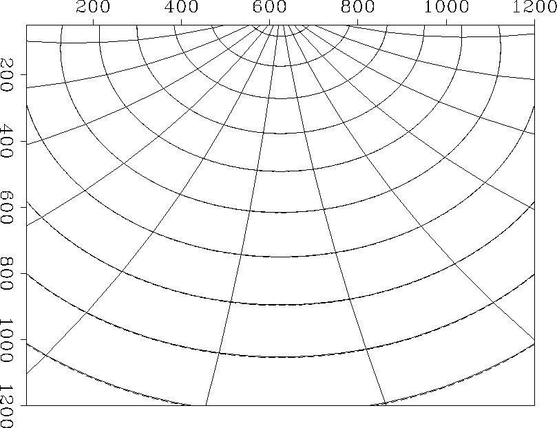
Figure 3 shows the numerical result from dynamic ray tracing and the theoretical solution. The ray tracing result agrees with the theoretical result satisfactorily.

 

model1 Figure 3 Solid lines represent numerical result (including ray and wavefront). The dash line represents theoretical result. The wavefront from ray tracing is consistent with the wavefront from equation (17). The raypaths also bend upwards because of the increase of velocity with depth.