


This section presents the results of applying
AMO prior to partial stacking,
to a marine data set recorded in the North Sea.
We compare the results of partial stacking after NMO and AMO,
with the results of partial stacking after simple NMO.
The data set is a valuable test case for AMO because
it shows numerous fault diffractions and because
proper imaging of it requires
3-D prestack depth migration Hanson and Witney (1995).
Figure ![[*]](http://sepwww.stanford.edu/latex2html/cross_ref_motif.gif) shows an in-line geological
section of the area of the survey and
the respective velocities of the layers.
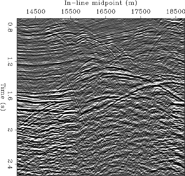
Figure shows a common-offset in-line
section of the data set, at the offset of 1 km.
The middle of the Jurassic layer, above the salt swell is highly faulted;
it creates the diffractions and fault reflections
visible in the middle of the section
between 0.8 and 1.2 s.
These reflections are affected by
shallow velocity variations created by variable thickness
in the low-velocity Tertiary sediments and
in a high-velocity Cretaceous chalk layer;
they are potential candidates for showing the advantages
of applying AMO prior to partial stacking.
The brighter reflectors at around 1.6 s
are generated at the salt-sediments interfaces.
The fairly steep reflections between 1.6 and 2 s,
at the left edge of the section,
are caused by the flanks of the salt swells.
These deeper reflections are affected not only by the shallow
velocity variations, but also by the high contrast in velocity between
the Jurassic and the Triassic layers.
shows an in-line geological
section of the area of the survey and
the respective velocities of the layers.
Figure shows a common-offset in-line
section of the data set, at the offset of 1 km.
The middle of the Jurassic layer, above the salt swell is highly faulted;
it creates the diffractions and fault reflections
visible in the middle of the section
between 0.8 and 1.2 s.
These reflections are affected by
shallow velocity variations created by variable thickness
in the low-velocity Tertiary sediments and
in a high-velocity Cretaceous chalk layer;
they are potential candidates for showing the advantages
of applying AMO prior to partial stacking.
The brighter reflectors at around 1.6 s
are generated at the salt-sediments interfaces.
The fairly steep reflections between 1.6 and 2 s,
at the left edge of the section,
are caused by the flanks of the salt swells.
These deeper reflections are affected not only by the shallow
velocity variations, but also by the high contrast in velocity between
the Jurassic and the Triassic layers.
 |


The data-acquisition configuration was double-source and triple streamer.
The nominal common-midpoint spacing was 9.375 m
in the in-line direction,
and 25 m in the cross-line direction.
The cable length was 2,200 m with maximum feathering
of approximately 17 degrees.
To make the data handling and processing quicker,
we processed only a subset of the whole data set.
We windowed in time the data traces up to 600
time-samples, for a maximum time of 2.4 s.
We selected the central 512 midpoints in the in-line direction,
for a total length of 4,800 m,
and 130 midpoints in the cross-line,
for a total width of 3,250 m.
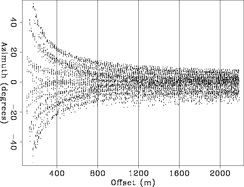
Figure shows the
offset-azimuth distribution of a small subset of the
data traces.
As it is typical for such acquisition geometry,
it shows six distinct trends,
most distinguishable at small offsets,
that correspond to each possible source-streamer pair.
 |
To test the effects of AMO on the prestack data, we applied two distinct partial stacking methods to the data: NMO followed by partial stacking (NMO-stacking); and NMO followed by AMO and partial stacking (NMO-AMO-stacking). To make the comparison as fair as possible to the conventional methodology of simple NMO-stacking, the traces after NMO were laterally interpolated in the midpoint direction before they were stacked into the output cube. Tests showed that this lateral interpolation preserved the dipping events significantly better than a simple binning procedure.
We applied partial stacking independently
on six different subsets of the data.
The subsets were determined according
to the absolute value of the offset.
Each offset range was 400 m wide, starting from zero.
The boundaries between the offset ranges are shown
as vertical bars in Figure .
For all offset ranges, the output data were a regularly sampled
cube with nominal offset equal to the midpoint of the range;
that is, 200, 600, 1,000, 1,400, 1,800 and 2,200 m.
The number of traces input into the partial-stacking process
depended on the offset range;
for example, for the 800-1,200 m range
the number of input traces was about 460,000.
The output cube had
512 midpoints in the in-line direction,
and 130 in the cross-line, for a total of
66,560 output traces.
Therefore, the data-reduction rate achieved
by partial stacking is approximately 7.
Before processing the data, we applied a hyperbolic mute with a sharp cut-off. To assure the removal of the first arrival and some severely aliased noise at the far-offset, we set the mute velocity slightly lower than water velocity. After muting, we applied NMO with a velocity function varying with midpoint and time. The NMO velocity function was given to us together with the data. No inverse NMO was applied to the results before they were plotted, thus the reflection timings are equivalent to ``zero-offset'' times. Of course, inverse NMO ought to be applied before the AMO results are input into a prestack depth migration. Because we do not yet have available a 3-D prestack Kirchhoff depth-migration program, we could not migrate the result of partial stacking. However, the prestack data results obtained by partial stacking show convincing evidence of the improvements obtained by including AMO in the process.
In general, the longer the offset
and the larger the azimuth rotation,
the more significant is the effect of AMO on the data.
For the geometry of our data set,
the most significant effects
are visible for the longer offset ranges,
starting from the 800-1,200 m range.
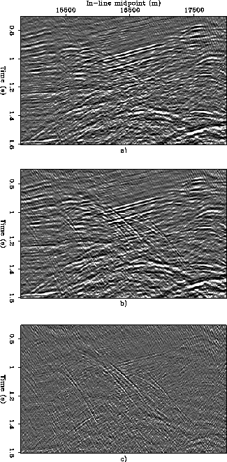
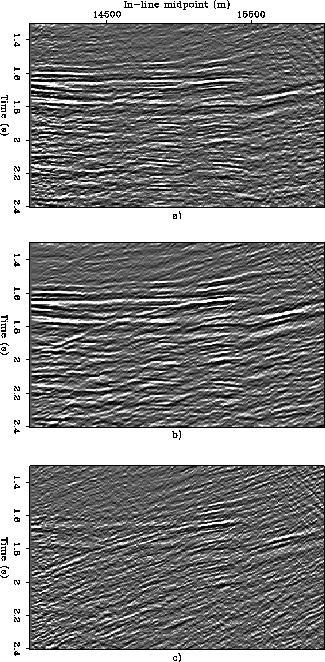
Figure compares the
results obtained with the two flows described above,
for the 800-1,200 m offset range.
The figure displays a window of an in-line section,
located at 19,590 m along the cross-line axis
and centered on the fault blocks
where the data show numerous high-frequency diffractions.
Figure a shows the section
obtained by simple NMO-stacking,
while
Figure b shows the
results of NMO-AMO-stacking.
As expected, the addition of AMO to the partial stacking
process preserves the diffractions much better
than simple NMO.
Figure c shows the differences between
the two sections;
diffractions and fault reflections are clearly evident.
 |
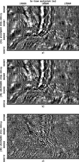
Figure
compares the time slices cut at 1.068 s,
for the same offset range (800-1,200 m)
as in Figure .
As in Figure ,
Figure a shows the results of NMO-stacking,
while Figure b shows the results of NMO-AMO-stacking.
The difference section (Figure c)
clearly shows that few trends of
high-frequency diffractions were not
correctly preserved by the conventional process.
The most evident differences tend
to occur for reflections that are oriented at an angle
with respect to the in-line direction.
This observation is consistent with
the fact that the conventional NMO-stacking
process is most inaccurate for
reflections that are oblique with
respect to the nominal azimuth;
the angle of maximum error is dependent on the reflector's dip.
Although there are not many such reflections in this data set,
which shows geological dips mostly aligned along
the in-line directions,
the AMO process enhances the ones that are present.
 |
Figure
compares the time slices cut at 1.1 s,
for the next offset range, that is, the 1,200-1,600 m range.
For this offset range, as in the previous one,
the trend of diffractions from
the fault blocks are strongly attenuated by the conventional
procedure of NMO followed by partial stacking.
On the contrary, AMO preserves these important events during
the stacking procedure.
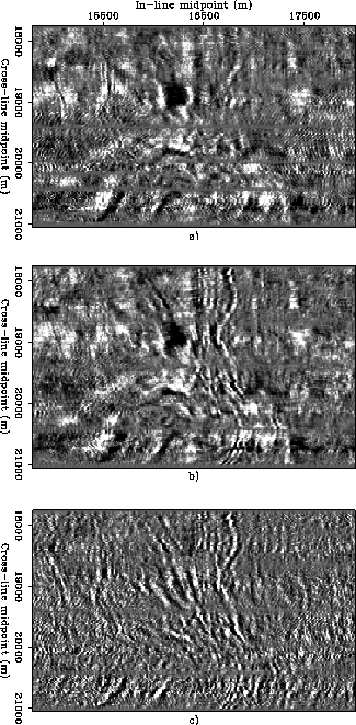 |
Figure shows windows of an in-line section
for the 1,200-1,600 m offset range.
This in-line section is located at 20,940 m and centered around
the salt-flank reflection visible
in the lower-left corner of Figure .
The dipping salt flank reflection
is better preserved by the application of AMO.
Further, as for the shallower section,
some mildly dipping reflections appear to
be ``cleaner'' after AMO.
A possible explanation for this phenomenon is that
the uncoherent stacking of the diffractions,
and of other steeply dipping reflections,
contributes to the general level of background noise
in the data obtained by simple NMO-stacking.
 |