

Next: Separation by 2-D spectral
Up: Separation by 1-D spectral
Previous: 1-D Separation theory
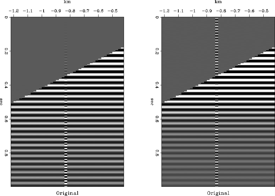
Figure ![[*]](http://sepwww.stanford.edu/latex2html/cross_ref_motif.gif) shows a very simple synthetic where the signal
is a constant frequency sine wave beginning at the start time
with an amplitude that varies as time squared.
The noise is also a constant frequency sine wave,
but has a different frequency than the signal.
The noise also has a constant amplitude instead of the t2 decrease
in amplitude seen in the signal.
There is a background of weak random noise.
shows a very simple synthetic where the signal
is a constant frequency sine wave beginning at the start time
with an amplitude that varies as time squared.
The noise is also a constant frequency sine wave,
but has a different frequency than the signal.
The noise also has a constant amplitude instead of the t2 decrease
in amplitude seen in the signal.
There is a background of weak random noise.
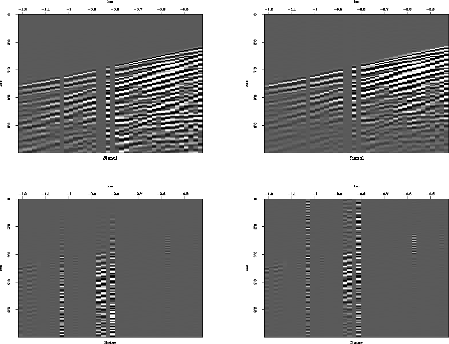
Figure ![[*]](http://sepwww.stanford.edu/latex2html/cross_ref_motif.gif) shows the result of predicting the
signal using equation (
shows the result of predicting the
signal using equation (![[*]](http://sepwww.stanford.edu/latex2html/cross_ref_motif.gif) ).
The trace that contained the noise is almost completely zeroed.
This zeroing was caused by the common effective null space of
the noise and signal filters.
In spite of the signal overwhelming the noise in the
area the signal filter was designed in,
the remaining noise was eliminated by the filter designed there.
When applied to the real shot data, the noisy traces are not
well separated, and the traces with noise are significantly weakened,
as seen in Figure
).
The trace that contained the noise is almost completely zeroed.
This zeroing was caused by the common effective null space of
the noise and signal filters.
In spite of the signal overwhelming the noise in the
area the signal filter was designed in,
the remaining noise was eliminated by the filter designed there.
When applied to the real shot data, the noisy traces are not
well separated, and the traces with noise are significantly weakened,
as seen in Figure ![[*]](http://sepwww.stanford.edu/latex2html/cross_ref_motif.gif) .
.
While other approaches may by taken, such as shortening the
filters or attempting to completely zero the noise before designing
the signal filter,
separation of signal and noise using one-dimensional filters
does not seem practical,
mainly because of the overlap of the null spaces created by
the signal and noise filters.
In the next sections,
I address these shortcomings by making the signal filter
two-dimensional.
sinefile
Figure 4
A simple synthetic showing noise and signal with different spectra.
The plot on the left has t2 scaling, the plot on the right does not.


sf1w.b
Figure 5
A simple example of separation of signal and noise using
sine waves of different frequencies.
The method of equation (![[*]](http://sepwww.stanford.edu/latex2html/cross_ref_motif.gif) ) was used.
The plot on the top is the calculated signal, and the plot on the
bottom is the noise that remained.
The plot on the left has t2 scaling, the plot on the right does not.
) was used.
The plot on the top is the calculated signal, and the plot on the
bottom is the noise that remained.
The plot on the left has t2 scaling, the plot on the right does not.


sf1w.a
Figure 6
A simple example of separation of signal and noise using
the real data from Figure 10.1.
The method of equation (![[*]](http://sepwww.stanford.edu/latex2html/cross_ref_motif.gif) ) was used.
The plot on the top is the calculated signal, and the plot on the
bottom is the noise that remained.
The plot on the left has t2 scaling, the plot on the right does not.
) was used.
The plot on the top is the calculated signal, and the plot on the
bottom is the noise that remained.
The plot on the left has t2 scaling, the plot on the right does not.


Next: Separation by 2-D spectral
Up: Separation by 1-D spectral
Previous: 1-D Separation theory
Stanford Exploration Project
2/9/2001
![[*]](http://sepwww.stanford.edu/latex2html/cross_ref_motif.gif) shows a very simple synthetic where the signal
is a constant frequency sine wave beginning at the start time
with an amplitude that varies as time squared.
The noise is also a constant frequency sine wave,
but has a different frequency than the signal.
The noise also has a constant amplitude instead of the t2 decrease
in amplitude seen in the signal.
There is a background of weak random noise.
shows a very simple synthetic where the signal
is a constant frequency sine wave beginning at the start time
with an amplitude that varies as time squared.
The noise is also a constant frequency sine wave,
but has a different frequency than the signal.
The noise also has a constant amplitude instead of the t2 decrease
in amplitude seen in the signal.
There is a background of weak random noise.


