


Next: 1-D Separation examples
Up: Separation by 1-D spectral
Previous: Separation by 1-D spectral
To improve the separation, more information is required.
Here I attempt to use the time spectrum of the signal and the noise
as the extra information.
In a manner similar to the process used to determine the amplitudes,
the spectrum of each trace is calculated from the data above
the first break,
where the data above the first breaks are assumed to be noise.
Each trace has a separate filter calculated.
For the noise, a single filter is derived over the data
after the first breaks.
The filters used here annihilate the signal and noise.
The signal filter is represented by
|  |
(117) |
where  is the scaled signal
and
is the scaled signal
and  is the matrix form of the filter.
A single filter is used for the signal in all traces.
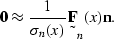
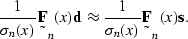
The noise filter appears as
is the matrix form of the filter.
A single filter is used for the signal in all traces.
The noise filter appears as
|  |
(118) |
 is a function of x because a separate filter is computed
for each trace.
For this section and the next,
the noise filter is calculated on the data above the start times.
In this section both these filters are one dimensional.
is a function of x because a separate filter is computed
for each trace.
For this section and the next,
the noise filter is calculated on the data above the start times.
In this section both these filters are one dimensional.
I would like to incorporate what I know about the amplitudes
of the signal and noise from section ![[*]](http://sepwww.stanford.edu/latex2html/cross_ref_motif.gif) with the filters derived
here to improve the separation of signal and noise.
Since the signal loses amplitude as about t2,
I multiply the signal by t2 and force the signal to zero
above the start time by
using the function T'(x,t,v), which varies as t2 below
the start time and is a large fixed constant above the start time.
The relative amplitudes of the noise and signal are also available
from section .
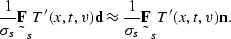
To minimize the signal and the noise together, I use
with the filters derived
here to improve the separation of signal and noise.
Since the signal loses amplitude as about t2,
I multiply the signal by t2 and force the signal to zero
above the start time by
using the function T'(x,t,v), which varies as t2 below
the start time and is a large fixed constant above the start time.
The relative amplitudes of the noise and signal are also available
from section .
To minimize the signal and the noise together, I use
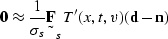
| 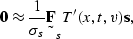 |
(119) |
and
|  |
(120) |
Modifying equation () using  gives
gives
|  |
(121) |
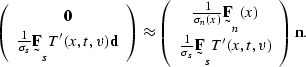
Expressing both systems as a single system gives
| 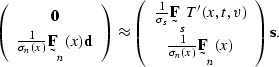 |
(122) |
An alternative approach is to solve for the noise.
By repeating the same set of steps, but solving for the noise instead
of the signal with  , equation () becomes
|  |
(123) |
or
|  |
(124) |
This expression, combined with equation (), gives
|  |
(125) |
The results of either system () or () may be used.
Appendix A of Abma 1994
shows that the results of either system of equations
will produce equivalent results when  ,but it can be seen that this does not apply when null spaces
containing the signal and noise occur.
Although it might be argued that the filters and are
never perfect and so actual null spaces are not created,
given a reasonable number of iterations of the least-squares solver
and the finite capabilities of the floating point number representation used,
effective null spaces will be created in these cases.
Since the filters and are fairly effective in
removing the noise and signal,
they create effective null spaces in systems () and ().
,but it can be seen that this does not apply when null spaces
containing the signal and noise occur.
Although it might be argued that the filters and are
never perfect and so actual null spaces are not created,
given a reasonable number of iterations of the least-squares solver
and the finite capabilities of the floating point number representation used,
effective null spaces will be created in these cases.
Since the filters and are fairly effective in
removing the noise and signal,
they create effective null spaces in systems () and ().
Another way of looking at this null space problem is to examine the
information that is available in the system to calculate a solution.
In system (),
any information about the noise is eliminated from the system
since the filter has removed the noise from the data going
into the left-hand side of the system.
Therefore, the signal calculated from system () will
not contain any information removed by .If any information in the signal falls in the null space created by
,the solution for the signal from system () will not contain
that information.
In system (),
any information about the signal is eliminated from the system
since the filter has removed the signal from the data going
into the left-hand side of the system.
Therefore, the noise calculated from system () will
not contain any information removed by .If any information in the noise falls in the null space created by
,the solution for the noise from system () will not contain
that information.
In short,
if the signal and noise have overlapping null spaces,
the overlap is eliminated in systems () and ().
Another aspect of solving these inversions involves
initialization of the inversionAbma (1995).
This initialization reduces the number of iterations of the
solver significantly, thus reducing the cost of the inversion.
It also modifies the action of the inversion.
If system () has the signal initialized with the original
data,
any data in the common null space create by and will not be
removed from the signal.
For system () initialized with the original data,
any data in the common null space create by and will not be
removed from the noise.
It can then be seen that the noise calculated from system ()
without initialization
subtracted from the data will be equal to the signal calculated from
system () with initialization.
Also, the signal calculated from system ()
without initialization
subtracted from the data will be equal to the noise calculated from
system () with initialization.
For one-dimensional filters,
the overlap of the action of and is likely
to be a problem, especially when both the signal and noise are
broadband.
One approach to solving the problem of this overlap is to
modify the systems so that the effective null spaces do not occur.
One method I have tried is to separate the amplitude and the filtering
effects into separate equations.
These equations were
|  |
(126) |
| |
(127) |
|  |
(128) |
and
| |
(129) |
Expanded with relative weights to predict the signal,
these minimizations become
the single system of regressions that follows:
| 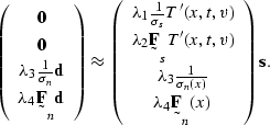 |
(130) |
This system has no effective null spaces.
Unfortunately, () and () assume that the signal and
noise are constant functions,
not the sinusoidal functions normally found in seismic data.
While system () worked well for the peaks of the noise and
signal, it failed near the zero crossings.
Because of these failures, I will no longer consider approaches
such as that in system ()
in this thesis.
Next: 1-D Separation examples
Up: Separation by 1-D spectral
Previous: Separation by 1-D spectral
Stanford Exploration Project
2/9/2001