

Next: Conclusions
Up: Distribution of events not
Previous: Event attenuation by weighting
Several cases are shown here that illustrate the effects
of the weighting in the previous discussion.
The first case shows the effects of varying  in
equation (
in
equation (![[*]](http://sepwww.stanford.edu/latex2html/cross_ref_motif.gif) ). Figure
). Figure ![[*]](http://sepwww.stanford.edu/latex2html/cross_ref_motif.gif) shows
the events from which the signal filter
shows
the events from which the signal filter  and the noise filter
  are calculated.
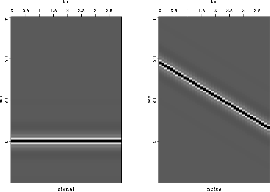
The data in Figure
 ![[*]](http://sepwww.stanford.edu/latex2html/cross_ref_motif.gif) are therefore taken as definitions
of signal and noise,
the signal being the flat event and the noise being the dipping event.
Figure
are therefore taken as definitions
of signal and noise,
the signal being the flat event and the noise being the dipping event.
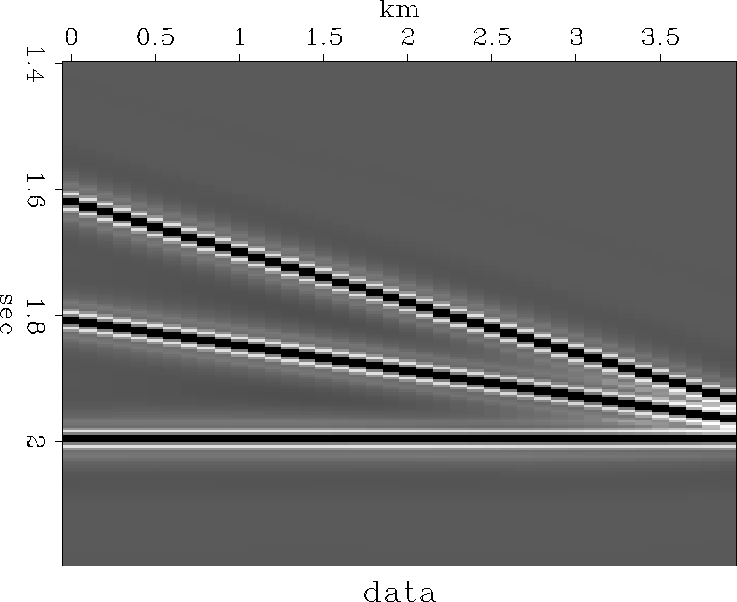
Figure ![[*]](http://sepwww.stanford.edu/latex2html/cross_ref_motif.gif) shows the data to be separated into signal and noise.
In addition to the signal and noise seen in Figure
shows the data to be separated into signal and noise.
In addition to the signal and noise seen in Figure ![[*]](http://sepwww.stanford.edu/latex2html/cross_ref_motif.gif) ,
an event with a dip of intermediate slope has been added
in Figure
,
an event with a dip of intermediate slope has been added
in Figure ![[*]](http://sepwww.stanford.edu/latex2html/cross_ref_motif.gif) .
This event is only slightly attenuated by the filters
.
This event is only slightly attenuated by the filters  and
and  .
.
By solving equation (![[*]](http://sepwww.stanford.edu/latex2html/cross_ref_motif.gif) ) with
) with  ,the results seen in Figure
 ![[*]](http://sepwww.stanford.edu/latex2html/cross_ref_motif.gif) are obtained.
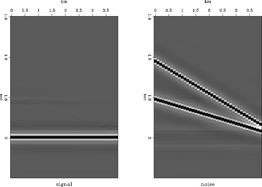
The event with the intermediate slope has been about evenly distributed
between the signal and the noise.
are obtained.
The event with the intermediate slope has been about evenly distributed
between the signal and the noise.
Next, equation (![[*]](http://sepwww.stanford.edu/latex2html/cross_ref_motif.gif) ) is solved with
) is solved with  .Increasing
  increases the weight given to the top part of
equation (
increases the weight given to the top part of
equation (![[*]](http://sepwww.stanford.edu/latex2html/cross_ref_motif.gif) ),
),  ,
so events that do not fit
  extremely well get eliminated from
  .As expected, Figure
 ![[*]](http://sepwww.stanford.edu/latex2html/cross_ref_motif.gif) shows the event
with intermediate slope has been almost completely moved to the noise.
shows the event
with intermediate slope has been almost completely moved to the noise.
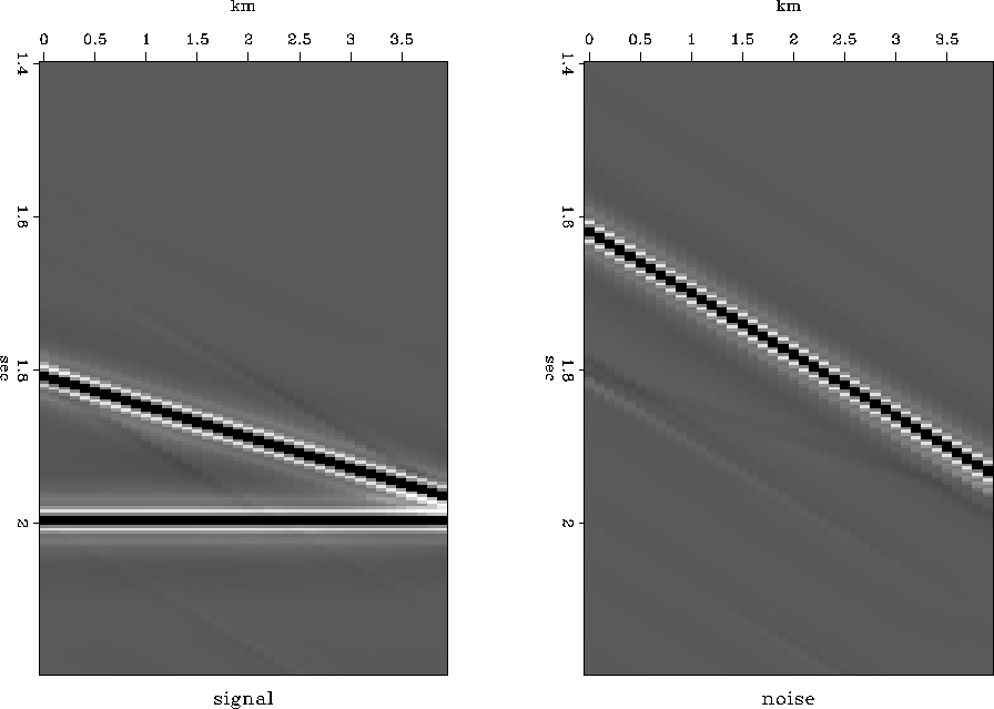
When  is decreased to 0.1,
the weight given to the top part of equation (
is decreased to 0.1,
the weight given to the top part of equation (![[*]](http://sepwww.stanford.edu/latex2html/cross_ref_motif.gif) ) is decreased
so any event that does not fit the lower part of equation (
) is decreased
so any event that does not fit the lower part of equation (![[*]](http://sepwww.stanford.edu/latex2html/cross_ref_motif.gif) )
extremely well is pushed into
)
extremely well is pushed into  .This can be seen in Figure
 ![[*]](http://sepwww.stanford.edu/latex2html/cross_ref_motif.gif) ,
where the event of intermediate slope is almost entirely
contained in the signal.
,
where the event of intermediate slope is almost entirely
contained in the signal.
signalnoise.a
Figure 7
The event on the left is defined as signal,
the event on the right is defined as noise.
|
|  |


data.a
Figure 8
The data, made up of both signal and noise, and an added event.
|
|  |


In the previous examples,
equation (![[*]](http://sepwww.stanford.edu/latex2html/cross_ref_motif.gif) ) has been solved with a zero estimated value
of
) has been solved with a zero estimated value
of  .This was possible since the signal was not significantly attenuated
by the filter
  .In the next examples,
equation (
.In the next examples,
equation (![[*]](http://sepwww.stanford.edu/latex2html/cross_ref_motif.gif) ) has been solved with a preliminary estimate
of
) has been solved with a preliminary estimate
of  being the data
  ,since both filters
  and
and  can completely eliminate one part of
the data.
For Figures
 ![[*]](http://sepwww.stanford.edu/latex2html/cross_ref_motif.gif) to
to ![[*]](http://sepwww.stanford.edu/latex2html/cross_ref_motif.gif) ,
the signal filter
,
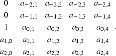
the signal filter  is a two-dimensional
prediction-error filter with the form
|  |
(97) |
The noise filter  is a one-dimensional
prediction-error filter with the form
|  |
(98) |
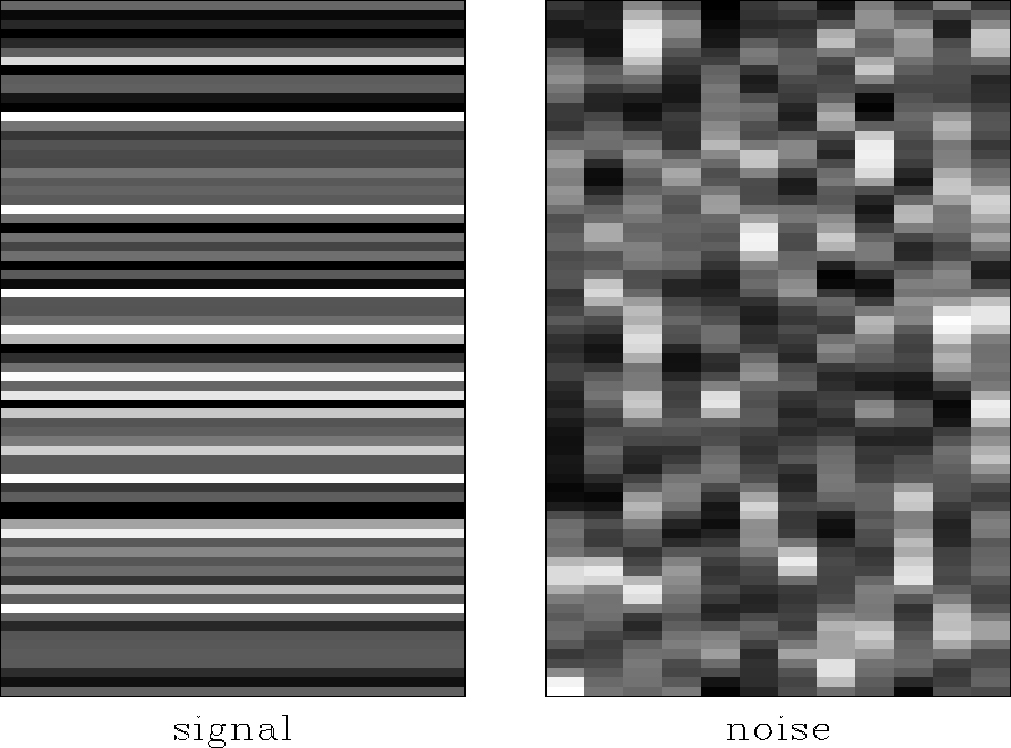
Figure ![[*]](http://sepwww.stanford.edu/latex2html/cross_ref_motif.gif) shows the events defined as the signal and noise.
The signal is a series of horizontal events with random amplitudes.
The noise is mono-frequency sine waves with random shifts.
Both filters (
shows the events defined as the signal and noise.
The signal is a series of horizontal events with random amplitudes.
The noise is mono-frequency sine waves with random shifts.
Both filters (![[*]](http://sepwww.stanford.edu/latex2html/cross_ref_motif.gif) ) and (
) and (![[*]](http://sepwww.stanford.edu/latex2html/cross_ref_motif.gif) ) will eliminate the sine waves,
since a prediction is done along the time axis,
but only filter (
) will eliminate the sine waves,
since a prediction is done along the time axis,
but only filter (![[*]](http://sepwww.stanford.edu/latex2html/cross_ref_motif.gif) ) can predict the signal,
since the amplitudes in time are random
and unpredictable by filter (
) can predict the signal,
since the amplitudes in time are random
and unpredictable by filter (![[*]](http://sepwww.stanford.edu/latex2html/cross_ref_motif.gif) ).
To allow any of the noise in the output,
equation (
).
To allow any of the noise in the output,
equation (![[*]](http://sepwww.stanford.edu/latex2html/cross_ref_motif.gif) ) must be solved with a preliminary estimate
of
) must be solved with a preliminary estimate
of  being the data, or all the sine waves will be removed from the system.
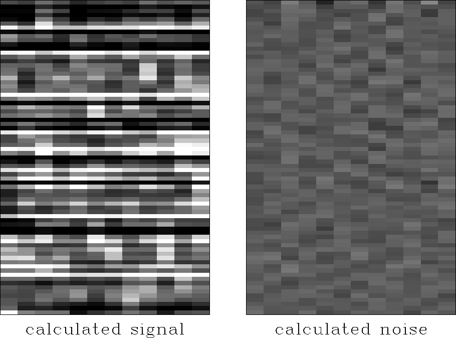
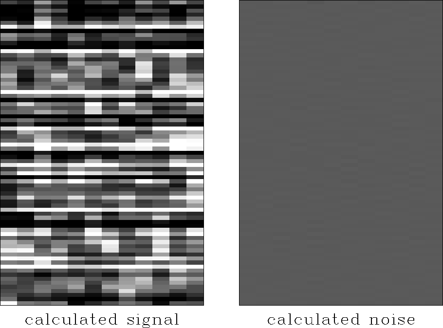
When equation (![[*]](http://sepwww.stanford.edu/latex2html/cross_ref_motif.gif) ) is solved with
) is solved with  ,Figure
 ![[*]](http://sepwww.stanford.edu/latex2html/cross_ref_motif.gif) shows that the noise is evenly distributed
between the calculated signal and the calculated noise.
Increasing
shows that the noise is evenly distributed
between the calculated signal and the calculated noise.
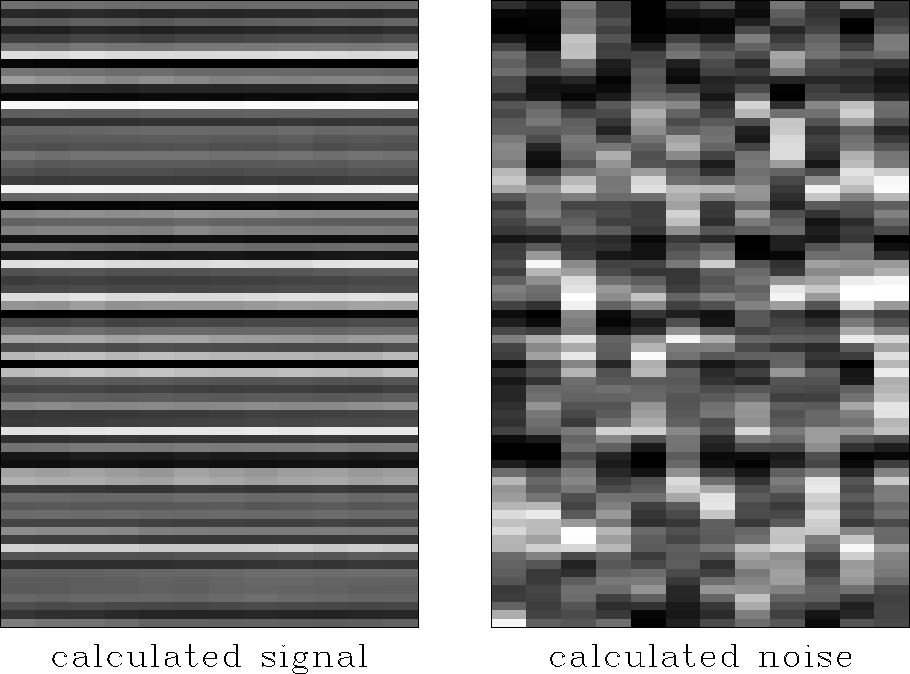
Increasing  to 10 moves the sine waves into the noise section,
producing the excellent separation of signal and noise
seen in Figure
 ![[*]](http://sepwww.stanford.edu/latex2html/cross_ref_motif.gif) .
Decreasing
.
Decreasing  to 0.1 moves the sine waves
almost completely into the signal.
This weighting gives a useful tool in distributing events
between calculated signal and noise.
input
Figure 12
The events on the left are defined as signal,
the events on the right are defined as noise.


signois.1
Figure 13
The calculated signal and noise using  .
.


signois.10
Figure 14
The calculated signal and noise using  .
.


signois.0.1
Figure 15
The calculated signal and noise using  .
.


Next: Conclusions
Up: Distribution of events not
Previous: Event attenuation by weighting
Stanford Exploration Project
2/9/2001
![[*]](http://sepwww.stanford.edu/latex2html/cross_ref_motif.gif) ). Figure
). Figure ![[*]](http://sepwww.stanford.edu/latex2html/cross_ref_motif.gif) shows
the events from which the signal filter
shows
the events from which the signal filter ![[*]](http://sepwww.stanford.edu/latex2html/cross_ref_motif.gif) are therefore taken as definitions
of signal and noise,
the signal being the flat event and the noise being the dipping event.
Figure
are therefore taken as definitions
of signal and noise,
the signal being the flat event and the noise being the dipping event.
Figure ![[*]](http://sepwww.stanford.edu/latex2html/cross_ref_motif.gif) shows the data to be separated into signal and noise.
In addition to the signal and noise seen in Figure
shows the data to be separated into signal and noise.
In addition to the signal and noise seen in Figure ![[*]](http://sepwww.stanford.edu/latex2html/cross_ref_motif.gif) ,
an event with a dip of intermediate slope has been added
in Figure
,
an event with a dip of intermediate slope has been added
in Figure ![[*]](http://sepwww.stanford.edu/latex2html/cross_ref_motif.gif) .
This event is only slightly attenuated by the filters
.
This event is only slightly attenuated by the filters 