

Next: Conclusions
Up: Three-dimensional lateral prediction
Previous: The three-dimensional extension of
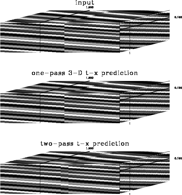
An example of the 3-dimensional prediction's ability
to predict nonlinear events
is shown in Figure ![[*]](http://sepwww.stanford.edu/latex2html/cross_ref_motif.gif) ,
where the input consists of several dipping layers cut by a fault
in the crossline direction,
so that events are nonlinear in the inline direction.
In the cubes in Figure
,
where the input consists of several dipping layers cut by a fault
in the crossline direction,
so that events are nonlinear in the inline direction.
In the cubes in Figure ![[*]](http://sepwww.stanford.edu/latex2html/cross_ref_motif.gif) and the figures that follow,
the vertical direction is the time axis, the horizontal direction
is the inline spatial axis,
and the direction running into the page is the crossline
spatial axis.
The lines on the cubes indicate the position of the slices shown on
the faces of the cube.
The one-pass 3-dimensional prediction did not smear the fault,
because the calculated 3-dimensional filter created a
prediction in the crossline direction that
preserved the discontinuity in the inline direction.
With the two-pass prediction, the inline pass
smeared the reflections across the fault.
For the noiseless case of Figure
and the figures that follow,
the vertical direction is the time axis, the horizontal direction
is the inline spatial axis,
and the direction running into the page is the crossline
spatial axis.
The lines on the cubes indicate the position of the slices shown on
the faces of the cube.
The one-pass 3-dimensional prediction did not smear the fault,
because the calculated 3-dimensional filter created a
prediction in the crossline direction that
preserved the discontinuity in the inline direction.
With the two-pass prediction, the inline pass
smeared the reflections across the fault.
For the noiseless case of Figure ![[*]](http://sepwww.stanford.edu/latex2html/cross_ref_motif.gif) ,
the f-x prediction is not shown because it gave the same results as
the t-x prediction.
,
the f-x prediction is not shown because it gave the same results as
the t-x prediction.
yplanesld
Figure 5
A comparison of smearing with one- and two-pass t-x prediction.
The top cube is the input,
the middle cube is the result of a one-pass 3-dimensional t-x prediction,
and the bottom cube is the result of two passes of one-dimensional
t-x prediction in the inline and crossline directions.
The one-pass result shows no smearing of the fault; the two-pass result
shows a smeared fault image.


The results of applying f-x prediction and t-x prediction
to a 3-dimensional
land survey provided by ARCO are
shown in Figures ![[*]](http://sepwww.stanford.edu/latex2html/cross_ref_motif.gif) to
to ![[*]](http://sepwww.stanford.edu/latex2html/cross_ref_motif.gif) to demonstrate the differences between
the two processes.
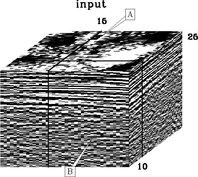
This data set is interesting because it has a significant noise level
with fairly flat, predictable events.
to demonstrate the differences between
the two processes.
This data set is interesting because it has a significant noise level
with fairly flat, predictable events.
Arcoorig
Figure 6
The input to the t-x and f-x predictions.
A significant amount of noise is seen here.
In this figure and the ones that follow, the vertical axis is time
and the horizontal axes are space.


For both two-pass applications,
the filter size was five elements in the spatial direction.
For both 3-dimensional one-pass applications,
I employed a filter with five elements in both spatial directions.
The t-x prediction used a five-element filter length in the time direction
for both one- and two-pass applications.
The window sizes were 60 traces in the inline
direction,
60 traces in the crossline direction,
and 200 samples, or 0.4 seconds in time.
Both the two-pass and the one-pass
t-x prediction results in Figures ![[*]](http://sepwww.stanford.edu/latex2html/cross_ref_motif.gif) and
and ![[*]](http://sepwww.stanford.edu/latex2html/cross_ref_motif.gif) show less noise than the corresponding f-x results;
otherwise the results are similar.
While the one-pass t-x prediction and f-x prediction results are much the same,
the t-x prediction output shows somewhat less noise.
show less noise than the corresponding f-x results;
otherwise the results are similar.
While the one-pass t-x prediction and f-x prediction results are much the same,
the t-x prediction output shows somewhat less noise.
Arcotx2d
Figure 7
The result of two passes of 2-dimensional t-x prediction processing.
While this result is an improvement over the input, some of the details
are seen to be lost when compared to the 3-dimensional t-x prediction.
More noise has been attenuated than with the two-pass f-x prediction.


Arcotx3d
Figure 8
The result of 3-dimensional t-x prediction processing.
This result preserves the details lost in the two-pass t-x prediction.


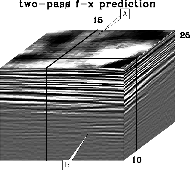
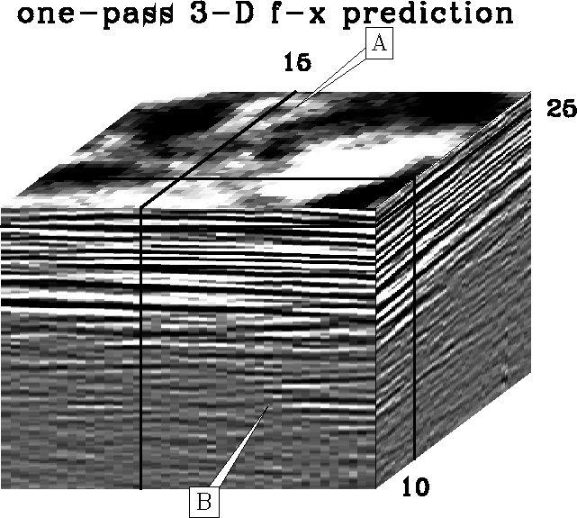
The advantage of using 3-dimensional lateral prediction is
especially clear in Figures ![[*]](http://sepwww.stanford.edu/latex2html/cross_ref_motif.gif) and
and ![[*]](http://sepwww.stanford.edu/latex2html/cross_ref_motif.gif) .
Both the one-pass results show significantly less smearing of the
structure. On the top faces of the cubes in Figures
.
Both the one-pass results show significantly less smearing of the
structure. On the top faces of the cubes in Figures ![[*]](http://sepwww.stanford.edu/latex2html/cross_ref_motif.gif) and
and ![[*]](http://sepwww.stanford.edu/latex2html/cross_ref_motif.gif) ,
the one-pass results appear clean and reasonable,
whereas the two-pass
results show smearing along the inline and crossline directions.
An example of the smearing of the detail can be seen at point A of these
figures, where a small doughnut-shaped feature is badly smeared in
both the two-pass results.
The front face of the cubes in Figures
,
the one-pass results appear clean and reasonable,
whereas the two-pass
results show smearing along the inline and crossline directions.
An example of the smearing of the detail can be seen at point A of these
figures, where a small doughnut-shaped feature is badly smeared in
both the two-pass results.
The front face of the cubes in Figures ![[*]](http://sepwww.stanford.edu/latex2html/cross_ref_motif.gif) to
to ![[*]](http://sepwww.stanford.edu/latex2html/cross_ref_motif.gif) are significantly different for the
one- and two-pass results;
with the one-pass results
showing much more detail.
The features at point B in the figures
once again demonstrate the loss of detail.
Although the differences between the
3-dimensional t-x and f-x results in Figures
are significantly different for the
one- and two-pass results;
with the one-pass results
showing much more detail.
The features at point B in the figures
once again demonstrate the loss of detail.
Although the differences between the
3-dimensional t-x and f-x results in Figures ![[*]](http://sepwww.stanford.edu/latex2html/cross_ref_motif.gif) and
and ![[*]](http://sepwww.stanford.edu/latex2html/cross_ref_motif.gif) are less than those between the 2-dimensional t-x and f-x results
in Figure
are less than those between the 2-dimensional t-x and f-x results
in Figure ![[*]](http://sepwww.stanford.edu/latex2html/cross_ref_motif.gif) ,
the results of the
3-dimensional t-x prediction appear slightly cleaner than
those of the 3-dimensional f-x prediction.
,
the results of the
3-dimensional t-x prediction appear slightly cleaner than
those of the 3-dimensional f-x prediction.
Arcofx2d
Figure 9
The result of two passes of 2-dimensional f-x prediction processing.
While this result is an improvement over the input, some of the details
are seen to be lost when compared to the 3-dimensional f-x prediction.


Arcofx3d
Figure 10
The result of 3-dimensional f-x prediction processing.
This result preserves the details lost in the two-pass f-x prediction.


Next: Conclusions
Up: Three-dimensional lateral prediction
Previous: The three-dimensional extension of
Stanford Exploration Project
2/9/2001
![[*]](http://sepwww.stanford.edu/latex2html/cross_ref_motif.gif) ,
where the input consists of several dipping layers cut by a fault
in the crossline direction,
so that events are nonlinear in the inline direction.
In the cubes in Figure
,
where the input consists of several dipping layers cut by a fault
in the crossline direction,
so that events are nonlinear in the inline direction.
In the cubes in Figure ![[*]](http://sepwww.stanford.edu/latex2html/cross_ref_motif.gif) and the figures that follow,
the vertical direction is the time axis, the horizontal direction
is the inline spatial axis,
and the direction running into the page is the crossline
spatial axis.
The lines on the cubes indicate the position of the slices shown on
the faces of the cube.
The one-pass 3-dimensional prediction did not smear the fault,
because the calculated 3-dimensional filter created a
prediction in the crossline direction that
preserved the discontinuity in the inline direction.
With the two-pass prediction, the inline pass
smeared the reflections across the fault.
For the noiseless case of Figure
and the figures that follow,
the vertical direction is the time axis, the horizontal direction
is the inline spatial axis,
and the direction running into the page is the crossline
spatial axis.
The lines on the cubes indicate the position of the slices shown on
the faces of the cube.
The one-pass 3-dimensional prediction did not smear the fault,
because the calculated 3-dimensional filter created a
prediction in the crossline direction that
preserved the discontinuity in the inline direction.
With the two-pass prediction, the inline pass
smeared the reflections across the fault.
For the noiseless case of Figure ![[*]](http://sepwww.stanford.edu/latex2html/cross_ref_motif.gif) ,
the f-x prediction is not shown because it gave the same results as
the t-x prediction.
,
the f-x prediction is not shown because it gave the same results as
the t-x prediction.


