


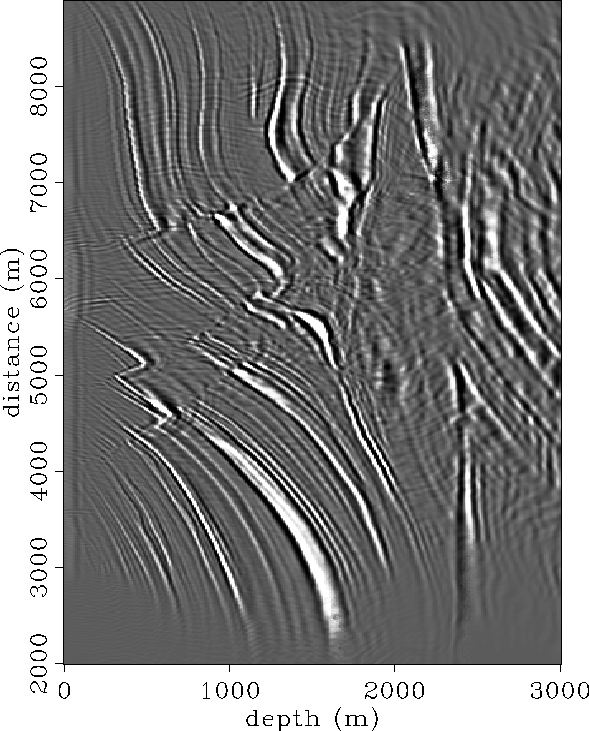
The last image of Figure ![[*]](http://sepwww.stanford.edu/latex2html/cross_ref_motif.gif) is displayed at full scale in
Figure . It is generated by downward continuing the data
to a depth of 1500 m in one datuming step. The downward
continued data are then migrated and combined with the previous image of
the upper 2000 m. This overlap is used to preserve image quality because
the portion of the image directly below the 1500 m datum suffers from the
effects of limited offset and near-field Kirchhoff distortion. The overlap
simply avoids the near-surface distortion suffered by most Kirchhoff
migration algorithms.
is displayed at full scale in
Figure . It is generated by downward continuing the data
to a depth of 1500 m in one datuming step. The downward
continued data are then migrated and combined with the previous image of
the upper 2000 m. This overlap is used to preserve image quality because
the portion of the image directly below the 1500 m datum suffers from the
effects of limited offset and near-field Kirchhoff distortion. The overlap
simply avoids the near-surface distortion suffered by most Kirchhoff
migration algorithms.
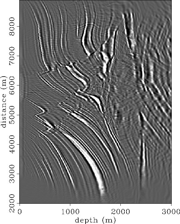
Figure is a clear improvement over the standard
migration displayed in Figure .
The anticlinal structure below the salt and the target are now clearly imaged.
An even greater imaging improvement is attained by making the datuming
step shorter since this insures that the first-arrival traveltimes
are a better approximation to the most energetic arrivals.
Continuation of the data to 1500 m in three steps of 500 m each, results
in an even better-focused
image of the anticline and the target (Figure ).
In both Figure and ,
the events which unconformably define the top of the anticline,
the anticline events themselves, and the target events are clearly
imaged. The lateral continuity and event coherency in the
target zone are substantially improved in Figure .
 |
![[*]](http://sepwww.stanford.edu/latex2html/movie.gif)


 |
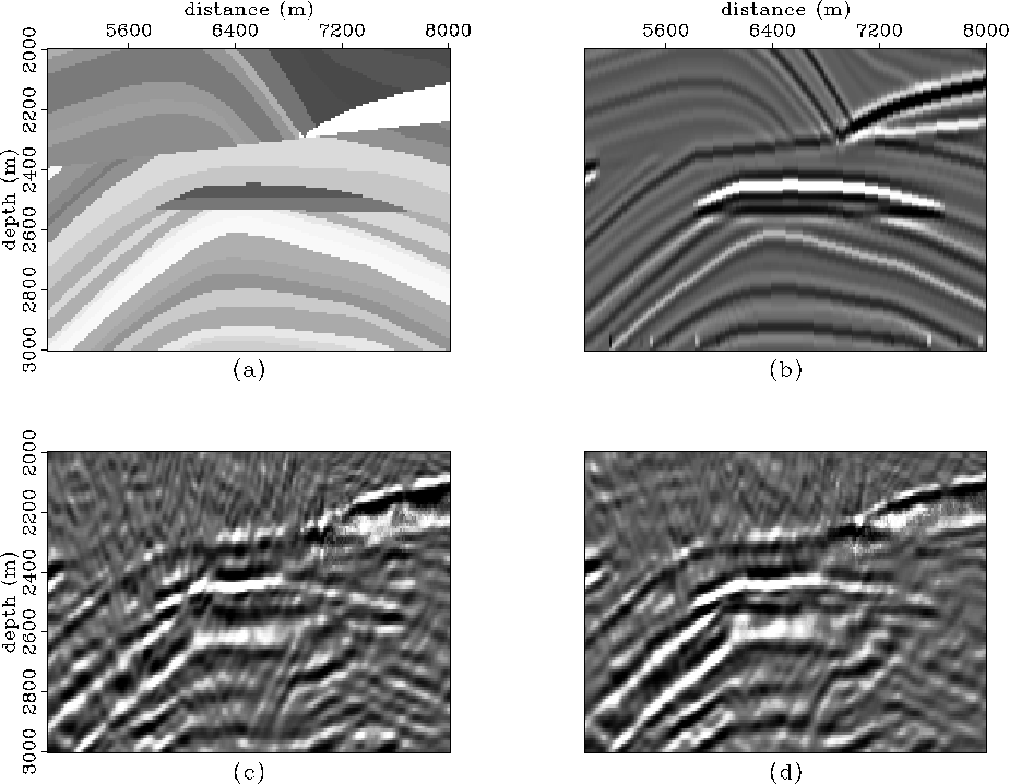
In Figure , I compare the images in the vicinity
of the target zone to the velocity model and a synthetic reflectivity
model which represents the desired image.
The synthetic reflectivity (Figure b) is obtained by
combining the velocity and density models and convolving with
a wavelet. This type of resolution cannot be expected from migration, but
ideally, the migration results should provide a
comparable structural image.
Both of the layer-stripping images in
Figures c and d
compare favorably with the desired reflectivity.
The image obtained by downward continuing the data in three steps
of 500 m is superior since the events display
better lateral continuity and the image is clearer.
This is because the traveltimes calculated for each of the 500 m steps
are better behaved than the traveltimes calculated
for one step of 1500 m. The resolution is so good that the
flat spot in the reservoir and the strongly reflective cap
stand out clearly. The phase of the events is a good match to that of the
synthetic reflectivity section.
 |