Searching the Sea of Galilee
The splendors and miseries of iteratively reweighted least squares

Sergey Fomel and Jon F. Claerbout

sergey@sep.stanford.edu, jon@sep.stanford.edu

As the former time made light the land of Zebulun and the land of Naphtali, so the latter hath honoured the way of the sea, beyond the Jordan, Galilee of the nations. Isaiah 9:1

ABSTRACT

We applied the inverse linear interpolation method to process a bottom sounding survey data set from the Sea of Galilee in Israel. Non-Gaussian behavior of the noise led us to employ a version of the iteratively reweighted least squares (IRLS) technique. The IRLS enhancement of the method was able to remove the image artifacts caused by the noise at the cost of a loss in the image resolution. Untested alternatives leave room for further research.

 

galgol
Figure 1 Map of the Sea of Galilee vicinity, grabbed from a state gopher site in Israel.

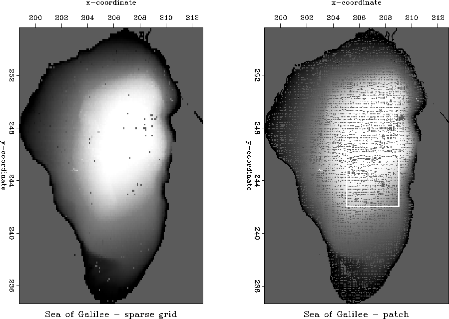
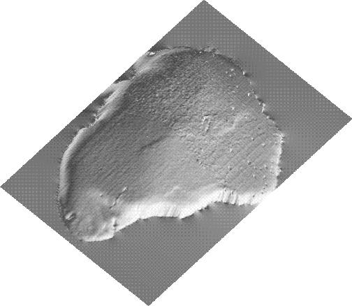
The Sea of Galilee, also known in Israel as Lake Kinneret (Figure galgol), is a unique natural object because of both its ancient history and its geography. It is a rare case of a freshwater lake below sea level. From a geological point of view, the location of the lake is connected to a great rift crossing east Africa. Our project addressed processing of the bottom sounding survey data collected by Zvi Ben Abraham at Tel-Aviv University .

The original data include over 100,000 triples (x_i,y_i,z_i) . The range of x's is about 12 km, and the range of y's is about 20 km. The depth coordinates range from 211 m to 257 m below sea level. Consecutive measurements are close to each other and cover the area of the lake with a fairly even grid. However, a number of empty bins remains even after sparse binning (Figure galsea). Using primitive preprocessing editing, we got rid of several measurements containing zeroes or evident mispositioning errors.

 

galsea
Figure 2 Sea of Galilee data after simple binning. On the left is a sparse grid (the size of a bin is about 100 by 100 m); on the right, a denser grid (50 by 50 m). The bordered square was chosen for the first set of experiments.

The major goal of this project was to interpolate the data to a regular grid. Properly interpolated data can enable searching for the local features of interest, including geological structures as well as sunken ships and other exotic archeological objects. Our attention was focused on developing a data interpolation technique that might be useful in a wide variety of geophysical applications.

The general method we chose for the problem is linear inverse interpolation with a known filter, as described by . This method did produce the desired result, but a non-Gaussian noise distribution caused serious problems in its implementation. To cope with these problems, a version of the iteratively reweighted least squares (IRLS) technique (, ) was applied.

METHOD: INVERSE LINEAR INTERPOLATION WITH KNOWN FILTER

The theory of inverse linear interpolation with a known filter is given in Applications of Three-Dimensional Filtering (), section 2.6, and can be easily extended to the 2-D case. The algorithm is based on the following procedure. To invert the data vector ${\bf d}$ given on an irregular grid for a regularly sampled model ${\bf m}$, we run the conjugate-gradient solver on the system of equations

$${\bf d \approx Lm\;, \EQNLABEL{linear} }$$ (1)

$${\bf 0 \approx \epsilon \, Am\;. \EQNLABEL{regression}}$$ (2)

Equation linear formulates the basic assumption of the method, stating that the data is related to the model with a linear interpolation operator ${\bf L}$. The next equation regression is required to constrain an underdetermined part of the inverse problem. Minimizing the output power of the model filtered by some roughening filter ${\bf A}$ is a way to smooth the model components that are not determined by equation linear. Laplacian filter of the form

$${\bf A}= \begin{array} {\vert c\vert c\vert c\vert} \hline .... ... 1 \\ \hline . & 1 & . \\ \hline\end{array}\EQNLABEL{laplacian}$$ (3)

is a conventional choice for smoothing in two dimensions.

FIRST RESULTS

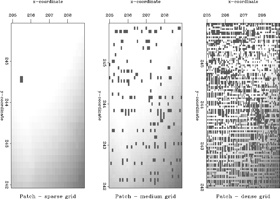
To test the inverse linear interpolation method, we cut a 4 by 4 km patch from the initial data plane and posed the problem of interpolating the data to a regular mesh. Figure galpat shows the patch after sparse, medium, and dense simple binning.

 

galpat
Figure 3 Simple binning of a patch. The left plot is the result of binning on a sparse grid (the size of a bin is 160 by 160 m); the right, on a denser grid ($40 \times 40$ m). The middle plot represents the medium case (80 by 80 m). Black spots are empty bins.

The result of the inverse linear interpolation on the dense grid after 200 iterations is shown in Figure gallap. For a better display, we convolve the interpolated data with a set of first-order derivatives, taken in different directions, such as:

$\begin{array} {cccc} \begin{array} {\vert c\vert c\vert} \hline 1 & . \\ \hline... ...rt c\vert c\vert} \hline . & -1 \\ \hline 1 & . \\ \hline\end{array}\end{array}$ .

 

gallap
Figure 4 Interpolation on the dense grid. The left plot is the initial result of the LS interpolation. The middle plot is the same result illuminated by a directional first-order derivative filter. The right plot is the illuminated result of the simple binning on a sparse grid.

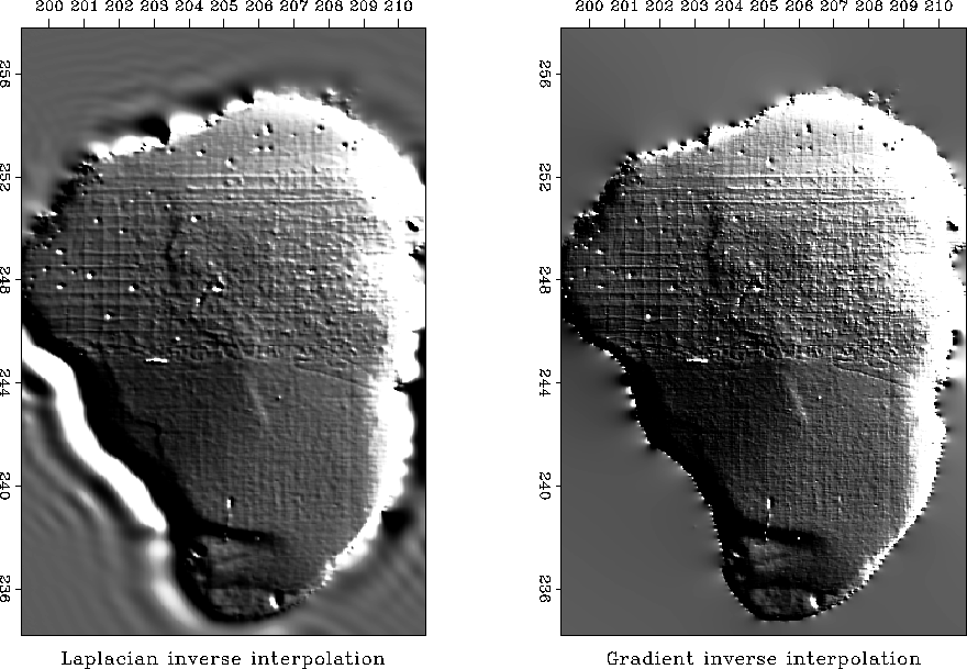
The result looks encouraging, since the interpolation produced a more detailed image than simple binning. However, this image is not satisfactory. Studying the sharp dipping discontinuity in the upper-right quarter of the patch revealed that it was produced not by a real geological structure but by an inconsistent track present in the data. The results of applying the interpolation technique to the whole lake bottom (the left side of Figure galsen) show more examples of that kind of noise and demonstrate that the problem of data inconsistency among different tracks is common for most parts of the lake.

Such an inconsistency is easily explained by taking into account the fact that the measurements were made on different days with different weather and human conditions. To allow for these circumstances, we had to reformulate the initial least squares optimization approach applied to inversion.

 

galsen
Figure 5 Sea of Galilee data after LS inversion interpolation. The left plot is the result of interpolation with a Laplacian filter; the right, of interpolation with a gradient filter.

ENHANCEMENTS OF THE METHOD: IRLS

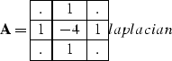
A minor improvement in the method was the change from the Laplacian filter laplacian in equation regression to the gradient filter consisting of the two orthogonal first-order derivatives

$${\bf A_1}= \begin{array} {\vert c\vert c\vert} \hline 1 & -1... ...e 1 \\ \hline -1 \\ \hline\end{array}\,\,. \EQNLABEL{gradient}$$ (4)

The reason for this change is evident in Figure galsen. The gradient filter is more appropriate for the sharp edges (the first-derivative jump) of the lake bottom, while the Laplacian filter tends to smooth them out. This fact is related to the close correspondence between gradient filter smoothing and local linear interpolation on one side, and Laplacian smoothing and cubic (spline) interpolation on the other.

The major enhancement is the introduction of a weighting operator ${\bf W}$ into equation linear. Thus system linear - regression takes the form

$${\bf 0 \approx W (d - Lm)}\;, \EQNLABEL{irls}$$ (5)

$${\bf 0 \approx \epsilon \, A_1 m}\;, \EQNLABEL{gradient1}$$ (6)

$${\bf 0 \approx \epsilon \, A_2 m}\;. \EQNLABEL{gradient2}$$ (7)

Though we didn't apply any formal straightforward theory to choose the weighting operator W, our heuristic choice followed two formal principles:

1.

Bad (inconsistent) data points are indicated by large values of the residual r = d - Lm left after conventional least squares inversion.

2.

Abnormally large residuals attract most of the conjugate gradient solver's efforts, directing it the wrong way. The residual should be whitened to distribute the solver's attention equally among all the data points and emphasize the role of the ``consistent majority.''

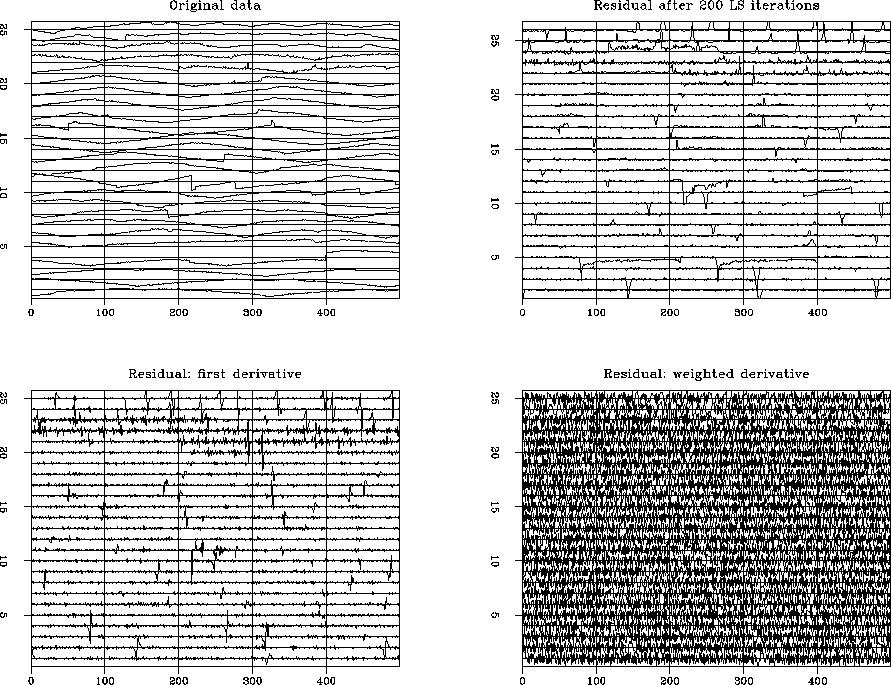
Figure galdat demonstrates changes in the residual space caused by the weighting. Each plot contains one long vector cut into several traces for better viewing. The top left plot is the original data from the patch used in the first experiments. The top right plot is the residual after 200 conventional conjugate gradient iterations. Note two major features of the residual distribution: statically shifted tracks (the zero-frequency component) and local bursts of energy (mostly in the upper part of the plot). To take away the zero-frequency component, we convolved the residual with the first-derivative operator. The result of differentiation appears on the bottom left plot. Finally, to take into account both large spikes created by differentiation and local bursts of energy, we constructed the following weighting function:

$$w_i = w(r_i) = {{2\,\bar{r}} \over {\mid r_i \mid + \bar{r_i}}} \,. \EQNLABEL{weight}$$ (8)

Here $\bar{r}$ stands for the median of the absolute residual values from the whole data set, and $\bar{r_i}$ is the median in a small window around a current point r_i. The denominator of the weighting function is designed to reduce the value of the residual if it belongs either to a spike (large $\mid r_i \mid$) or to a local burst of energy (large $\bar{r_i}$). The numerator was chosen for scaling purposes. The bottom right plot in Figure galdat justifies our choice of the weighting function, displaying the residual derivative after weighting. The signal distribution resembles white noise in accordance with the second formal principle.

 

galdat
Figure 6 View from the data space (explanation in the text).

Thus the weighting operator ${\bf W}$ in equation irls includes two components: the first-derivative filter ${\bf D}$ taken in the data space along the recording tracks and the weighting function w. Since w depends upon the residual, the inversion problem becomes nonlinear, and the algorithm approaches the IRLS class ().

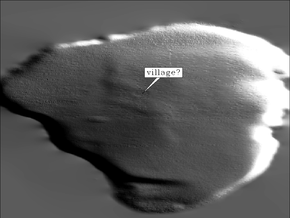
The result of the IRLS inversion is shown in Figure galrep. While the noisy portions of the model disappeared as we had expected, a large-scale structure (valley) crossing the lake from north to south remained on the image. Comparison of Figures galavl and galavn demonstrates that the price for that improvement is a certain loss in the image resolution. This type of loss occurs because we rely on the model smoothing to remove the noise influence. The role of the smoothing increases when we apply IRLS in the manner of piece-wise linearization. The first step of the piece-wise linear algorithm is the conventional least squares minimization. The next step consists of reweighted least squares iterations made in several cycles with reweighting applied only at the beginning of each cycle. Thus the problem is linearized within a cycle, and the conjugate gradient solver opens each cycle with the steepest descent iteration. What happens when the nonlinear reweighting is applied on each iteration is shown in Figure galres. Round ``villages'' on the bottom of the lake were identified as the consequence of occasional erroneous data points.

 

galrep
Figure 7 Result of the IRLS inverse interpolation (piece-wise linear).

 

galres
Figure 8 Result of the IRLS inverse interpolation (nonlinear).

DISCUSSION

The method of inverse linear interpolation with IRLS enhancement was able to produce a fairly clear image of the Sea of Galilee bottom, showing large-scale, presumably geological structures. The lessons learned from the Sea of Galilee project include the following:

• If a model (interpolation result) contains sharp edges, it can be preferable to use a gradient filter instead of a Laplacian one for smoothing purposes.
• The iteratively reweighted least-squares approach is capable of removing non-Gaussian noise influence on the result of inversion.
• The conjugate-gradient solver can behave differently in nonlinear and piece-wise linear implementations of nonlinear problems.

The main cause of the regular noise in the Galilee data set is the inconsistency among repeated measurements. An alternative approach could be applied to the problem of the data track inconsistencies. A well-known example of such an approach is the seismic mis-tie resolution technique (). Combining a technique of this kind with the inverse linear interpolation is a possible direction for future research.

Another interesting untested opportunity is preconditioning. As Bill Harlan has pointed out, the two equations in the system linear - regression contradict each other, since the first one aims to build details in the model, while the second tries to smooth them out. Applying the model preconditioning method could change the contradictory nature of the algorithm and speed up its convergence. The inversion problem takes the form

$${\bf 0 \approx W (d - LBx)} \EQNLABEL{precon}$$ (9)

$${\bf 0 \approx \epsilon \, x} \,\,\,,\EQNLABEL{nograd}$$ (10)

where ${\bf m=Bx}$, and ${\bf B}$ is a smoothing operator (an approximate inverse of the roughening operator ${\bf A}$ in regression). Possible advantages of preconditioning deserve special investigation.

 

galavl
Figure 9 Result of the LS inverse interpolation plotted in AVS.

 

galavn
Figure 10 Result of the IRLS inverse interpolation plotted in AVS.

[MISC,SEP,SEGCON,GEOPHYSICS,paper]