![[*]](http://sepwww.stanford.edu/latex2html/prev_gr.gif)
Sean Crawley
sean@sep.stanford.edu
INTRODUCTION
Land seismic data often shows large variations in energy from one trace to the next. Localized noise bursts or changes in signal to noise ratio in a shot gather, for instance where the receiver spread nears a road or machinery, are not uncommon problems. Also, geophones may be poorly coupled in an area, because of surface conditions or simply having been kicked loose. Claerbout points out in addition that local wavefields add amplitudes rather than energy. This means that wave interference can result in anomalously high or low trace energy where waves add or extinguish.
Typically, traces are scaled to have equal energies or equal mean absolute values. In situations such as those above this is not a perfect solution. In the case of noisebursts or machinery, reflection events may be given variable amplitudes depending on the amount of noise in individual traces when they should be constant along many traces. Or where events have extinguished, the resulting drop in initial trace power will result in noise being scaled up. Claerbout suggests that using a prediction error filter to destroy plane waves is perhaps a better way to estimate scales. In other words, scale traces based on the amplitudes along events rather than by total trace power or amplitude. When the proper filter is known, power in the output from locally planar data is minimized when the magnitude along events of a given dip is easily predictable, i.e. constant or smoothly increasing or decreasing.
Unfortunately, the scale anomalies we seek to solve for make the data less predictable, and the correct filter cannot be estimated from the input. I use a nonlinear technique to simultaneously solve for the scale factors and the filter. The inversion is unstable and conjugate gradient solutions typically diverge, but in general this occurs after a good solution has been reached.
Below I describe first the formulation of the problem, and afterwards the patches that enable the program to output good results despite divergence.
THEORY
Given locally monoplanar data, NMO corrected gathers for instance, a prediction error filter of n + 1 columns will completely extinguish planes at n dips. In the case where individual traces are incorrectly scaled, factors to rescale the traces may be estimated by solving the regression:
![]()
Rescaling the data changes the degree to which it is predictable, so the filter must be reestimated along with the scale factors. Thus the regression is rewritten:
![]()
![]()
Calculating the residual r to be ADs, the gradient directions for A and s are
![]()
![]()
One important consideration is the shape of the filter. For this problem, the shape of the filter is chosen to be (assuming one dip direction):

The regression has the trivial answer s=0. To avoid this, the condition
![]()
Low frequency artifacts
Least squares inversions are effective at removing large singular errors. Low frequency trends, however, are more difficult. Frequently this method produces outputs with spurious low frequency amplitude variations along events. I have found that simply scaling the columns in the filter will solve this problem, but this forces amplitudes to be constant along events, which is a mistake if we wish to preserve any AVO effects which may be present in the data. Instead, using the criterion that low frequency amplitude variations should come from the data and not from the scale factors, and assuming that scale anomalies are randomly distributed in space, we can filter the vector of scale factors with a filter of the form:
![]()
![]()
The added regression does a good job of supressing low frequency artifacts,
though in some cases it does inhibit the overall ability of the method to deal
with single large scale anomalies. Because the code takes very little
time to run (seconds to a minute for the example presented below), I
apply it two or three times in succession with decreasing values of ![]() .This application of the method has shown significantly reduced susceptibility to low
frequency artifacts in the examples I have tested.
.This application of the method has shown significantly reduced susceptibility to low
frequency artifacts in the examples I have tested.
Divergence
In every test I have run with this method on synthetics, the problem has eventually diverged. This is not very surprising when one considers the degree to which the scale factors and filter coefficients depend on one another, and the fact that both are found simultaneously. Several minor adjustments to the conjugate gradient solver make it slightly more robust, and make it possible to extract the best answer reached before divergence, rather than the final answer.
The first of these modifications is a change from our normal implementation of the conjugate gradient approach to one that resets when it runs into trouble. That is, in the event that after any iteration the residual has increased rather than decreased, one iteration of steepest descent is performed. This eliminates the contribution of the "bad" (meaning it resulted in increased residual power) previous solution direction to subsequent iterations. Also, I have employed a weighting parameter that factors the solution step length calculated by the conjugate gradient solver. Using smaller step lengths than those calculated by the solver (which are based on certain assumptions of linearity), increases slightly the stability of this nonlinear problem. Together these two changes tend to result in an inversion that reaches a smaller residual, but do not manage to stabilize it completely. A better solution is reached, but the problem still diverges at some time afterwards.
The most important adjustment to the conjugate gradient method is the addition of a buffer of a size to hold the solution and the value of the residual power associated with it. At each iteration, the residual power is computed, and if it is lower than that currently held in the buffer -the lowest value to that point in the inversion- the new solution is copied into the buffer. At the end, it is the contents of this buffer that are used to scale the input data. Finally, since repeated iterations of steepest descent means that the problem is diverging, a flag is used to abort after a given number of steepest descent iterations in a row.
RESULTS
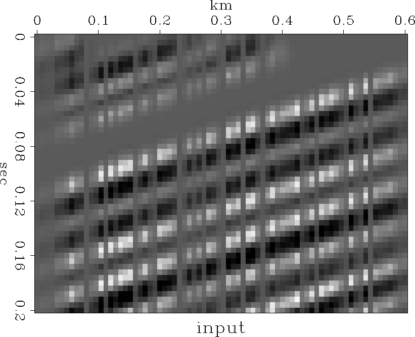
To test the algorithm, I applied random weights between one and 100 to each
trace in a
plane of data windowed from the Sigmoid synthetic data () .
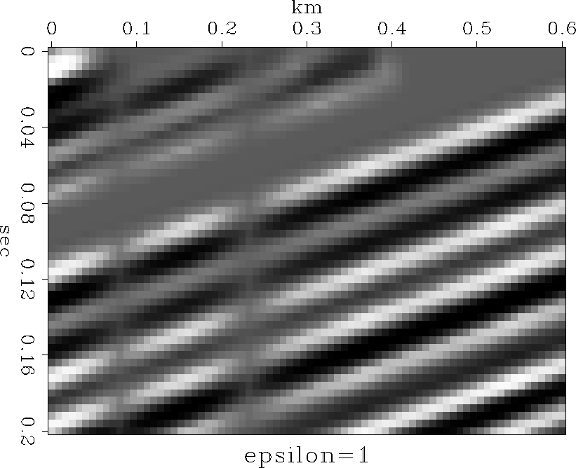
The input is displayed Figure input. After one pass through the
inversion with ![]() set to a value of one, the output is as seen in
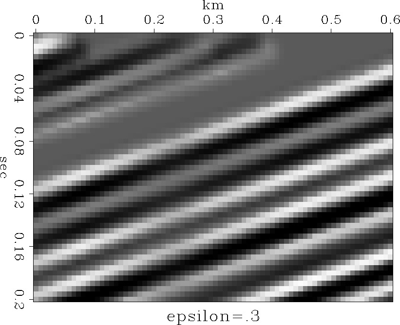
Figure output1. A second pass through the inversion with smaller
set to a value of one, the output is as seen in
Figure output1. A second pass through the inversion with smaller ![]() yields the result shown in Figure output3 .
yields the result shown in Figure output3 .
|
input
Figure 1 Randomly scaled input. Apparent missing traces are actually scaled by a small number. |  |
|
output1
Figure 2 Output after inversion with |  |
|
output3
Figure 3 Output after inversion with |  |
CONCLUSIONS
The results obtained on the synthetics are quite good. In addition, conversation with Bill Harlan led me to consider the possibility that this method can be extended to simultaneously solve for scale factors and static shifts, common problems with land seismic data. I plan to pursue this new problem in the future.
ACKNOWLEDGEMENTS I benefited from helpful conversations with Jon Claerbout, Matthias Schwab, and Bill Harlan. Also, the synthetics used for testing and display come from Jon's book, Three-Dimensional Filtering.
[sean,SEP,MISC]
![[*]](http://sepwww.stanford.edu/latex2html/prev_gr.gif)