THEORY

Claerbout formulates the inversion for this type of problem as follows. The first requirement for the output is that it should fit the input, the known data. This can be expressed as the regression

$$d \approx Lm$$

where d is the data, L is the linear interpolation operator that moves between model space and data space, and m is the model. This leads us to calculate a data residual r_d:

r_d = d - Lm

The second requirement is that the model should be consistent everywhere with the known data. We can estimate a prediction error filter and require that the model fit the filter with a regression of the form

$$0 \approx Am$$

where m again represents the model and A is the prediction error filter. This leads us to write the model residual:

r_m = -Am

However, we must estimate the filter from the model, which is the thing that we are inverting for. This means that we must find the model and the filter simultaneously. Rewriting A as $A + \Delta A$and m as $m + \Delta m$, the regressions become

$$d-L(m+\Delta m) \approx 0$$

$$-(A+\Delta A)(m+\Delta m) \approx 0$$

or

$$-Am \approx A\Delta m + M\Delta a$$

$$d-Lm \approx L\Delta m$$

The gradient directions for the filter and model are then

$$\Delta m = L'r_d + A'r_m$$

$$\Delta a = M'r_m$$

and the solution is obtained using conjugate gradients.

PREVIOUS WORK

Claerbout has used this method with a single grid (a model 160 points on a side) and achieved a good result, which can be seen in Figure levint . This result displays the qualities we would like to see in the output model. That is, the ridge segments in the sparsely sampled right portion of the survey area have been connected without smearing them terribly, and in the more densely sampled part of the survey area, it is hard to tell where data is known and where it is interpolated. Convergence, however, is slow. This result takes about 300 cpu minutes to generate running on our HP 700. Also, we may wish for a model with more structure and less smoothing away from the known data.

 

levint Figure 3 Nonlinear interpolation by Jon Claerbout. Model is 160 by 160 points, after 7,000 iterations.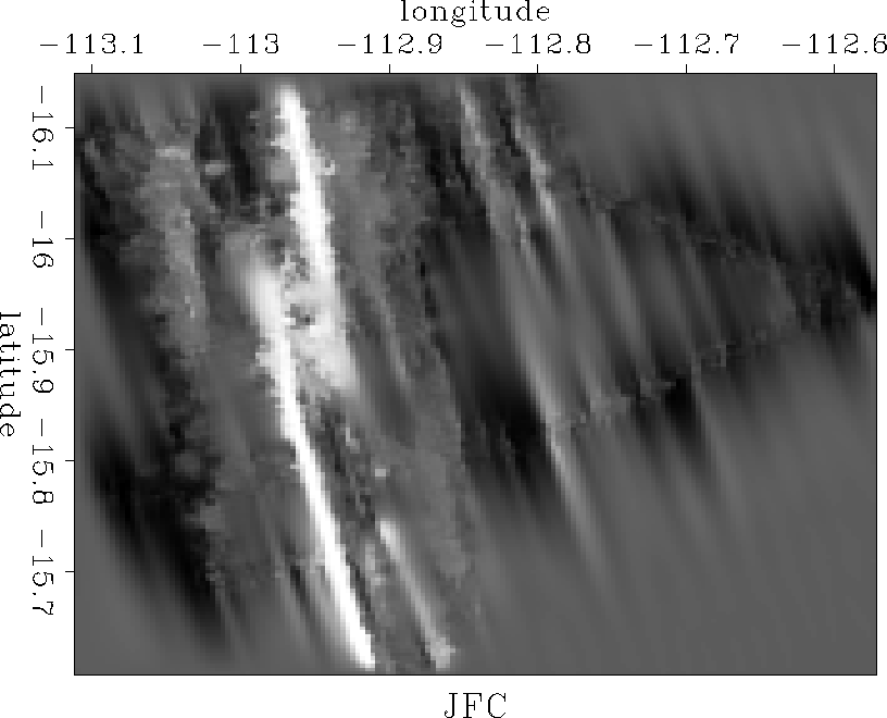

MULTIGRID

The model M can be chosen to have any number of points within the practical limitations of the data. The multigrid approach taken here is to begin by inverting for a very coarse model, with just 20 points on a side, and use the output as the initial guess for a more detailed model (the 20 by 20 model is pixel zoomed to become a 40 by 40 model, each bin being divided into four), and in this way gradually obtaining more detailed models. This serves several purposes. First, information is propagated into large unknown areas more quickly; the large unknown areas visible in Figure ras18 correspond to only a few tens of model points in the early stages of the problem. Second, because the filter isn't scaled up or down with the model, it operates on a range of spatial frequencies - the physical space occupied by the filter decreases as the number of points in model space increases. Thus large scale features and trends are resolved early in the inversion, and smaller scale features are overlaid. The workings of this are well illustrated by results displayed in Figures out2020 through out160160.

A further potential benefit of the multigrid approach is the avoidance of local minima. The simpler, early models should have smooth (low frequency) objective functions, enabling the solution to get close to the global minimum without becoming trapped in a local minimum. The solution then has a shorter distance to travel along the more convoluted and hazardous (higher frequency) objective functions of the later, more complex models. Of course, nothing guarantees that this leads to the true global minimum, but it should do at least as well or better than a normal gradient method ().

Windowing

An important consideration in using multigrid for this type of problem is how to window the measured data. The data residual, r_d, and the change in the data residual with each iteration are vectors the size of the data space, which for the entire data is 400,000 points. These vectors are used by the conjugate gradient solver to calculate step lengths, making iterations computationally expensive even on small grids where convolutions are quick and easy. Luckily, with a small number of bins in model space, a much reduced data set will suffice, and the early stages of the multigrid inversion can be solved in a few minutes. Of course, windowing too severely is dangerous. Obviously careless windowing creates the risk that important information in the data may be thrown out. I also found that with too severe a windowing strategy the algorithm actually became unstable and the residual exploded. This is important because it tells us the disastrous results (which I haven't bothered to display) are not the correct result to the wrong problem; the overwindowed data actually breaks the solver. In my own cursory examination, the critical number of data points has coincided with the number required to fill all the bins in model space in areas where there is known data. In addition, particularly when inverting for models with few and thus large bins, it is probably a good idea to include enough data to place many points in each bin, since there are likely to be a wide range of values present and a reasonable average is called for.

For this report, the full data set was used for the final model, mainly because windowing resulted in many empty bins near the edges of the areas where data was collected. For smaller models, the data were windowed to every thirteenth point. More severe windowing is of course possible. A more sophisticated approach, windowing more where several of the ship's tracks cross and less or not at all where there is a single track, would likely be an improvement in that it would make possible computationally easier iterations without losing information where there is little to begin with.

NEW RESULTS

The multigrid interpolation scheme was run on the SeaBeam data, beginning with a 20 by 20 model, the number of model points on a side doubling periodically up to 160. Results at each scale are displayed in Figures out2020 through out160160.

 

out2020 Figure 4 Model output on a 20 by 20 point grid after 1000 iterations.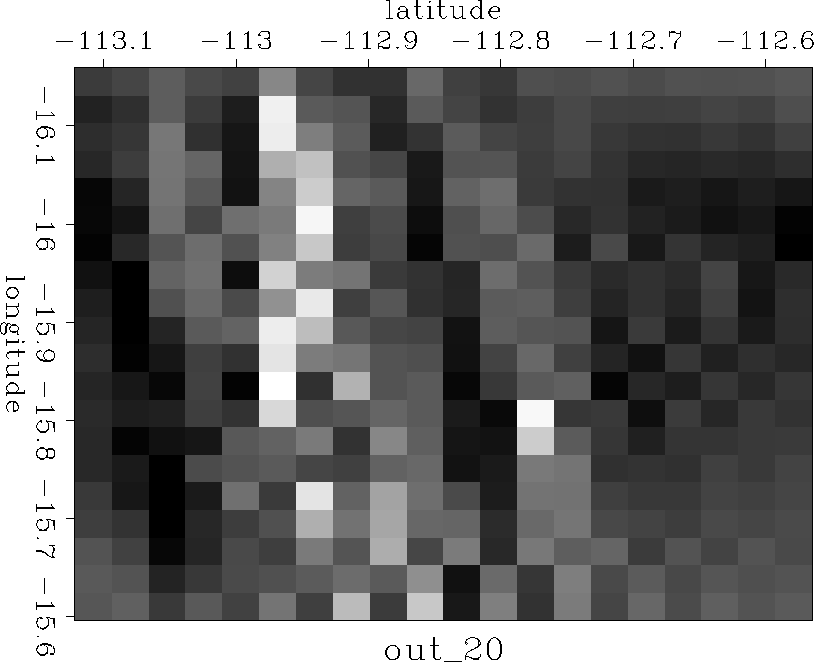

 

out4040 Figure 5 Model output on a 40 by 40 point grid after 3000 iterations.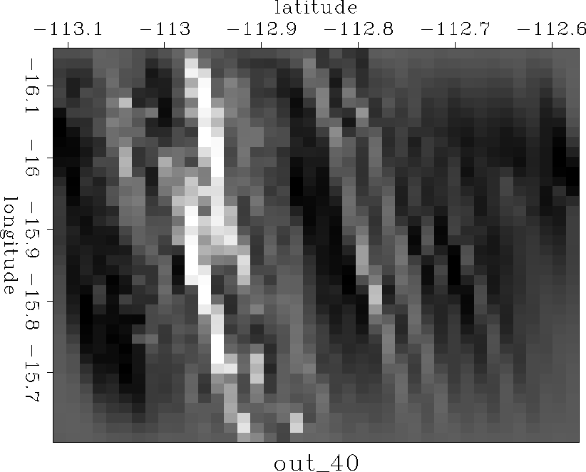

 

out8080 Figure 6 Model output on a 80 by 80 point grid after 3000 iterations.

 

out160160 Figure 7 Model output on a 160 by 160 point grid after 250 iterations.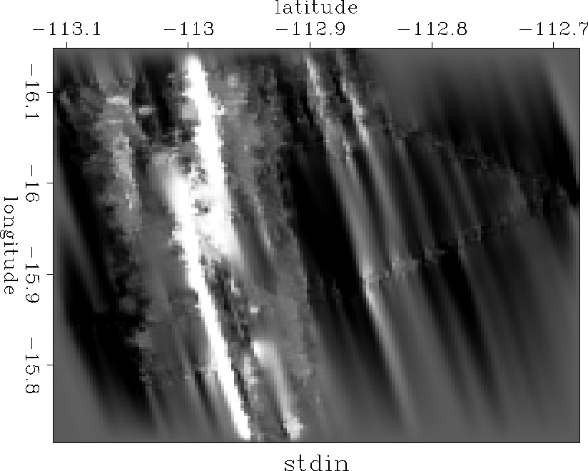

EVALUATION

To evaluate the performance of the multigrid method we compare Figures levint and out160160, the first done on a single grid and the second on multiple grids. The first observation is that the solutions are not identical. Ultimately, the two solutions are found with the same optimization criteria, the only difference being what we assume is a better starting guess in the multigrid case. In a nonlinear problem such as this, the starting solution may affect the final answer. Further, I believe that the multigrid method produced the more pleasing image. It appears more geologic and does not damp as severely towards the edges of the model. Of course, accuracy is hard to quantify because we are dealing with interpolated missing data. Still, the model produced by the multigrid inversion more closely approximates what we imagine the real sea floor to look like.

There is a definite difference in convergence speed. Though a similar total number of iterations was used in each case, multigridding allows most of the iterations to be performed at lower cost, thanks both to judicious windowing of the data space (smaller vectors in the solver), and fewer points in the model space to be convolved over. Convergence for the single grid inversion, Figure levint, took over 300 cpu minutes, while the same size model was solved for by the multigrid inversion in about one fifth the time, using the same machine and adjusting for cpu usage. Plots of residual power as a function of iteration for the single and multigrid inversions are displayed in Figure rescomp.

 

rescomp
Figure 8 Total residual power as a function of iteration for a single grid interpolation (left) and the final stage of a multigrid interpolation (right). Plots are clipped to a value of 1000 for clarity.

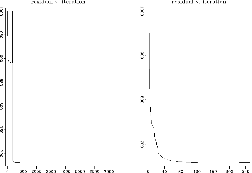The residual plots show some surprising things. For instance, there is a spike in the residual of the single grid interpolation that does not appear in the multigrid residual. This doesn't prevent the single grid inversion from converging to a good solution in this case, but may point to better stability for the multigrid method. More interesting is the speed with which the residual power appears to converge, particularly in the single grid case. It has stabilized after fewer than 1000 iterations, yet plotting the output after this many iterations, or even 3000 or 5000, yields a model that is a long way from being fully interpolated. In other words, small changes in residual energy can represent large changes to the model. Mathematically, this makes sense because the portion of the residual which represents the raw data (r_d = d-Lm) converges as soon as the model matches the raw data, which does not take very long. The remainder of the residual, r_m, exists due to filtering, and whether the bins are empty or contain interpolated values that fit the filter, this will have little power.

With the multigrid approach, stopping the inversion as soon as the residual has stabilized yields an output with more information in the model space, particularly in the sparsely covered right portion of the survey area. Comparing Figures levint and out160160 shows that the interpolated ridges have more continuity away from the measured data in the multigrid case. The model looks geological even close to its edges, where the single grid interpolation output damps away to zero. I think this is the effect of interpolating at multiple spatial frequencies, the larger scale features (the ridges) are better interpolated on a model with fewer points, where the filter is large enough to deal with them. Interestingly, carrying the last stage of the multigrid interpolation for several thousand iterations yields an image indistinguishable from that produced by the single grid inversion after a similar number. Both methods will eventually smear the model severely. The fact that both inversions degrade the model after very long runs points to a global minimum for our optimization criteria that is not really in line with our desires for the model. It is possible that improvements might yet be made by modifying the objective function for the problem.

CONCLUSIONS

There were several goals motivating the use of the multigrid approach in this problem. The first was speed. Convergence for this problem without multigrid took at least 300 cpu minutes; with multigrid and judicious use of windowing to take full advantage of the ease of solving of early grids with relatively few points in model space, about an hour. In this the method can be termed a success.

In addition, in cases where the data has different dominant frequencies, it appears that the multigrid method is better at finding a good output model because it can separate the frequencies. A possible further example and area for future work, is statics corrections in an area where the weathering layer thickness exhibits multiple dominant frequencies: for instance a general thickening trend as well as rapid local morphological variations.

A second goal is enhanced stability. The multigrid method has the potential to avoid local minima and thus converge to a better solution than is possible on a single grid. In this case the problem converged without real mishap on a single grid, so the greater robustness of the multigrid method wasn't tested.

ACKNOWLEDGEMENTS I benefited from conversations with Jon Claerbout and Matthias Schwab. I would also like to acknowledge Hector Urdaneta, with whom I worked in the early stages of this report.

[sean,SEG,MISC,EAEG,GEOTLE,geophysics]