Tomographic velocity estimation with planewave synthesis imaging

Jun Ji

jun@sep.stanford.edu

ABSTRACT

In areas with structurally complex geology, tomographic velocity analysis is required to estimate velocities. This paper describes a tomographic velocity analysis algorithm which uses planewave synthesis imaging as a prestack migration. In reflection tomography, prestack migration is required for both event picking and traveltime error computation. Traveltime errors are often measured in the form of residual moveout (RMO) velocity in common surface location (CSL) gathers after prestack depth migration. It is shown that we can measure the residual moveout (RMO) velocity accurately with the help of reflector-dependent planewave synthesis imaging.

The goal of processing seismic reflection data is to convert a recorded wave field into a structural or lithological image of the subsurface. Among the many steps in seismic processing, the imaging step, migration, positions reflector images. Migration requires a model of the wave propagation velocities of the subsurface, but obtaining this model is often the most difficult processing step in areas of complex structure.

In areas with structurally complex geology, conventional velocity analysis based on the stacking velocity (, ) often fails. Thus a more accurate velocity estimation scheme such as seismic tomography is required. Seismic tomography is an iterative two-step process. First, traveltime errors are measured by comparing observed traveltimes with computed traveltimes through an assumed velocity model. Then the differences are projected back over the traced ray paths through the assumed velocity model to update the model.

There are many different algorithms in tomographic velocity analysis, which can be characterized according to the domains they use for traveltime error picking. Conventional traveltime tomography (, ) picks the traveltime errors in the prestack data. Perhaps the greatest drawback of traveltime tomography of this type is the necessity for large amounts of picking. Events in seismic data are generally complicated and variable wave patterns; reducing this information to isolated time picks can involve large amounts of human judgement and can be very time consuming. The picking process is subject to systematic errors caused by ambiguities in defining events or by incorrect assumptions about the wavelet phase, as well as random error. Automatic picking programs can work faster than people, but human judgement is usually better at avoiding egregious mispicks.

In order to reduce the number, errors, and bias of picking, the semblance velocity stack panel can be used for picking. Since a pick of the best stacking velocity corresponds to a pick of the best-fitting hyperbolic traveltime for an event in the common-midpoint (CMP) domain, it can be interpreted as a filtered version of prestack traveltime picking ().

The results of those two types of the time domain picking can be achieved similarly in the image domain after prestack migration by picking events for every offset () or by picking the best residual moveout (RMO) velocity along the events in the stacked images (, ). In contrast to transmission tomography, where ray endpoints are known, in reflection tomography the reflector positions are unknown, and incorrectly guessing them may lead to errors in velocity estimation. Picking in the image space after prestack migration has the advantage of providing an accurate reflector location under the assumed velocity.

Tomographic velocity inversion constitutes a nonlinear inversion problem because both the velocity and ray paths are unknown. To solve such a nonlinear problem, we use a bootstrap approach. First, starting with an initial guess and the operator based on it, the traveltime errors are measured by comparing observed traveltimes with the computed traveltimes obtained through the assumed model. Next, the error in the assumed model is solved by inverting the measured traveltime errors. We then iterate this linear inversion with the updated velocity model until it converges.

If we choose the RMO velocity analysis for traveltime error measure, a model-dependent RMO velocity analysis is required to compute accurate traveltime error. However, the measuring of the RMO velocity for a nonflat reflector is often difficult and not practical to implement because it requires line search in a prestack migrated image cube (). To avoid such exhaustive searching, Etgen applied residual dip moveout (RDMO) before RMO velocity analysis so that the common reflection events could be lined up in the common surface location plane in the image cube.

This paper describes a way of measuring RMO velocity that reflects traveltime errors along the ray paths where the event has moved, with the help of planewave synthesis imaging along irregular reflectors. First, the paper reviews the basic traveltime tomography algorithm along with specific problems in reflection tomography. Then it explains how wavefront synthesis along irregular reflectors is used to generate reflector-oriented common reflection point (CRP) gathers, which provide accurate residual velocity. Finally, I summarize the whole algorithm for velocity estimation and show some examples.

REFLECTION TOMOGRAPHY

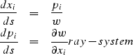
Traveltimes are a line integral of the slowness along the ray path expressed as

$$t = \int_s w ds,$$ (1)

where w is the slowness along the ray path, and s is the arc length along the ray path. With the slowness field discretized into cells, the forward problem of the traveltime is expressed as

$${\bf t} = L {\bf w}, \EQNLABEL{tomo-frd-nonlinear}$$ (2)

where ${\bf t}$ is a vector of traveltimes, ${\bf w}$ is a vector of slowness, and L is a matrix in which a row contains the path lengths of a ray in each cell. This forward problem is a nonlinear equation because the operator L depends on the slowness vector ${\bf w}$.

This nonlinear problem can be linearized by subtracting a reference problem and expressing the forward problem of the traveltime deviations from the reference model as follows:

$$\Delta {\bf t} = L \Delta {\bf w}, \EQNLABEL{tomo-frd-linear}$$ (3)

where $\Delta {\bf t}$ is a vector of traveltime deviations predicted from the reference model, $\Delta {\bf w}$ is a vector of slowness deviations from the reference model, and L is a matrix in which a row contains the path lengths in each cell of the ray traced through the reference model. For a given traveltime deviation, $\Delta {\bf t}$, the slowness deviation from the reference model, $\Delta {\bf w}$, is obtained by inverting equation tomo-frd-linear using the least-squares approach.

In order to solve the original nonlinear problem  tomo-frd-nonlinear, the above linearized inversion is applied iteratively with the updated back projection operator L_i, which is obtained by ray tracing through the new reference slowness

$${\bf w}_i = {\bf w}_{i-1}+\Delta {\bf w}_{i-1}$$ (4)

until the traveltime deviations $\Delta {\bf t}$ become small enough; the subscript i represents the number of iterations.

Therefore, traveltime tomography can be summarized as an iterative two-step process. First, traveltime deviations are measured by comparing picked traveltimes with expected traveltimes obtained through an assumed velocity model. Then the differences are projected back over the traced ray paths through the assumed velocity model to update the model.

In contrast to standard traveltime tomography, in which computation of the operator L only requires a slowness model to trace rays, reflection traveltime tomography requires additional information about reflectors, such as the dip and location. Therefore, an image space after prestack migration that can provide both the reflector information and the traveltime deviation is a good choice for picking.

MEASURING $\Delta {\bf t}$

The first step in traveltime tomography is measuring traveltime errors. For a given reference velocity model and reflector geometry, one can calculate traveltimes from each source to each receiver. Then traveltime errors are calculated by comparing the picked event with calculated traveltimes. Therefore, event picking is a prerequisite for measuring traveltime errors.

Event picking

The domain for picking plays a major role in deciding the type of tomography algorithm. Different algorithms use different domains for picking, such as the time or the depth in prestack or poststack, respectively. Among these picking algorithms, I chose the algorithm that picks events in the stacked image after prestack migration, which requires a minimum number of picks and provides reflector information. The advantage of having reflector information in the algorithm based on event picking in the depth domain is achieved by prestack migration. For this research, I used planewave synthesis imaging that synthesizes planewaves at the surface.

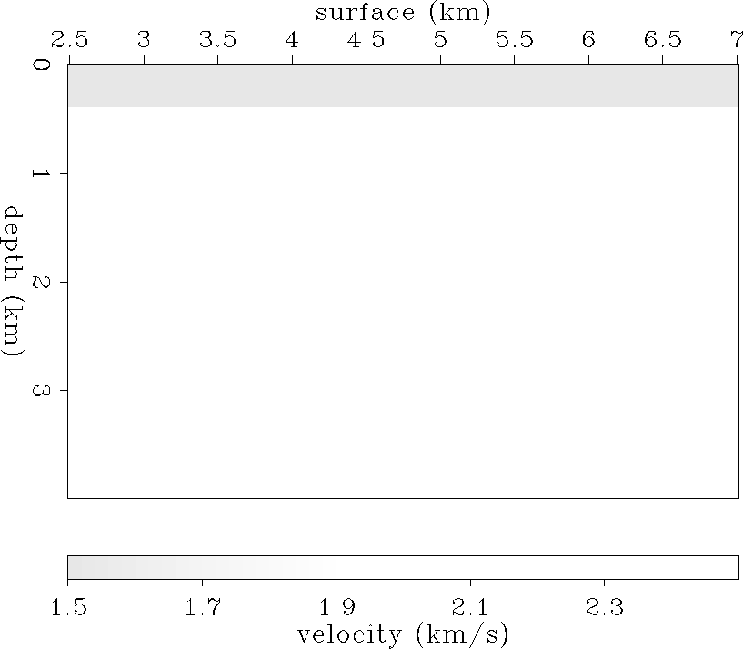
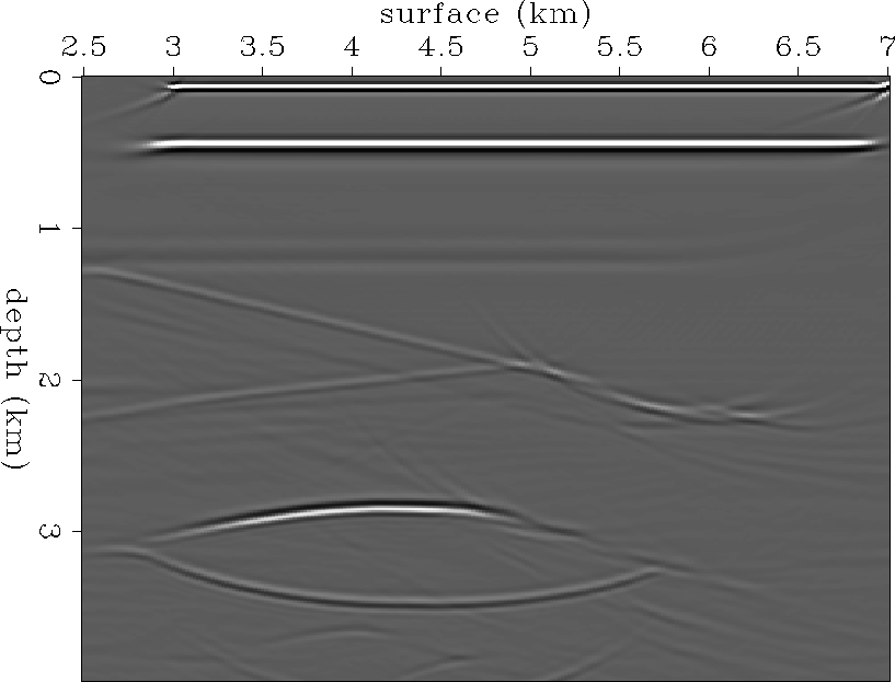
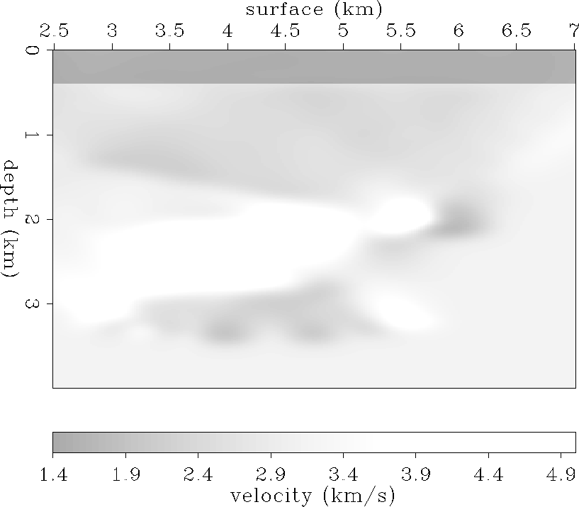
As an example, I have generated a synthetic data set with finite-difference acoustic modeling. Figure synvel shows an interval velocity model used to generate the synthetic data. To avoid surface-related multiples, I used an absorbing boundary at the surface. The near-offset section, Figure syn-near, shows that the multiples have been successfully suppressed.

As an initial guess for the velocity of the medium, a two-layer model, shown in Figure synvel-iter0, is used, with water velocity for the top layer because we can easily estimate the depth of the water bottom from the seismic data even in a real case.

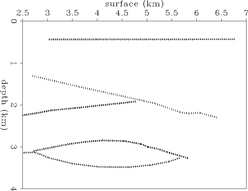
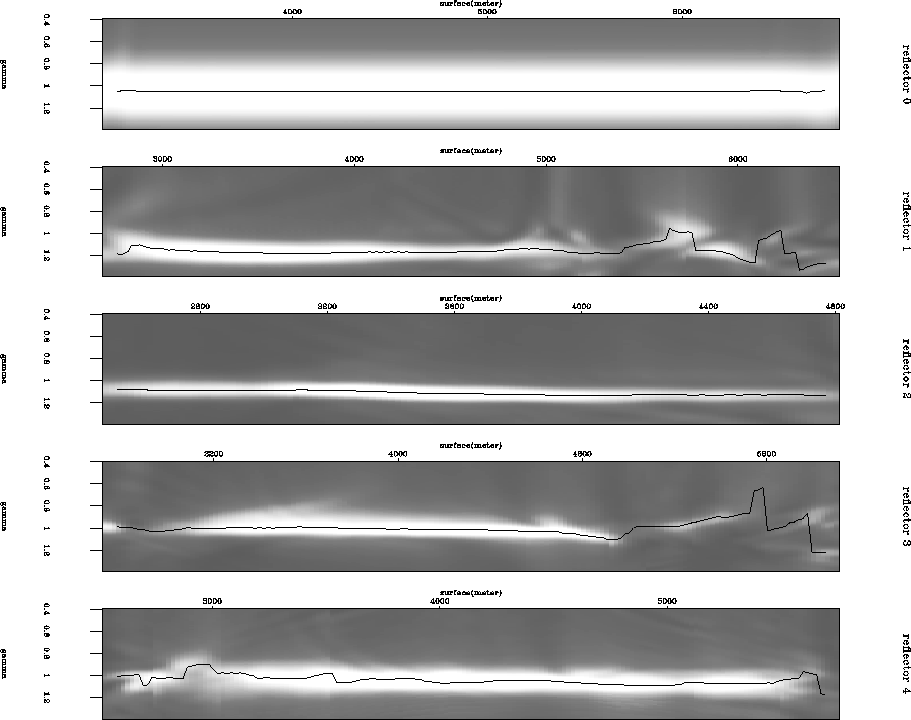
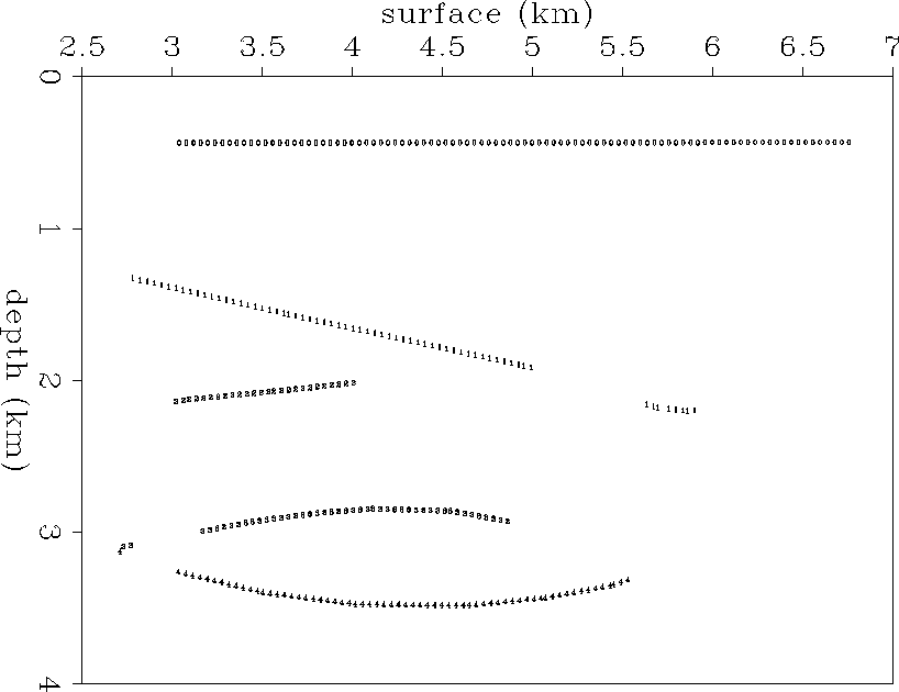
In order to obtain a reference image to pick dominant reflectors, I apply surface-oriented planewave synthesis imaging. I synthesized 31 different incidence angles at the surface; the stacked image of them all is shown in Figure pws-syn-iter0. Figure pick0 shows the locations of the reflectors picked, with reflector numbers assigned along them.

 

synvel
Figure 1 Velocity model used to generate a synthetic data set with finite-difference acoustic modeling.

 

syn-near
Figure 2 Near-offset section modeled using the finite-difference method.

 

synvel-iter0
Figure 3 Velocity model used as an initial guess. The top layer has a water velocity with the same thickness as that of the true model, and the lower layer has a velocity of 2.5 km/s.

 

pws-syn-iter0
Figure 4 Stacked image after planewave synthesis imaging that synthesized 31 different incidence angles, from -30 to +30 degrees, at the surface.

 

pick0
Figure 5 The picked reflectors. The numbers along each reflector represent the reflector number assigned.

RMO velocity analysis

Traveltime error computation along the event picked in the poststack image requires RMO velocity analysis. Measuring RMO implies relative movement of the event in the common reflection point (CRP) gathers according to different travel paths.

Conventionally, RMO velocity analysis is performed in the common surface location (CSL) gather after prestack migration. The RMO velocity obtained from the CSL gather after prestack migration does not reflect the correct residual movement of CRP images because CRP images are not lined up in CSL gathers when a reflector has a dip. Therefore, we need to apply residual dip moveout (RDMO) before RMO velocity analysis of CSL gathers () or else apply a dip-dependent RMO velocity analysis that is very difficult to implement ().

Even though surface-oriented planewave synthesis imaging also shows residual moveout in CSL gathers, it is not easy to quantify in terms of residual velocity. This is due to the lack of the information about the implied ray trajectories. Since both the source and the received wave field used in planewave synthesis imaging are plane waves, we do not know which source and receiver locations correspond an image. Therefore we update the model in a qualitative way using the curvature of the RMO curves ().

This drawback can be overcome by using reflector-oriented planewave synthesis imaging. With this method, the local incidence angle on top of the reflector is predefined. Thus, the image obtained can be interpreted as a wave field that follows the ray trajectory extended from the local incidence angle to the surface.

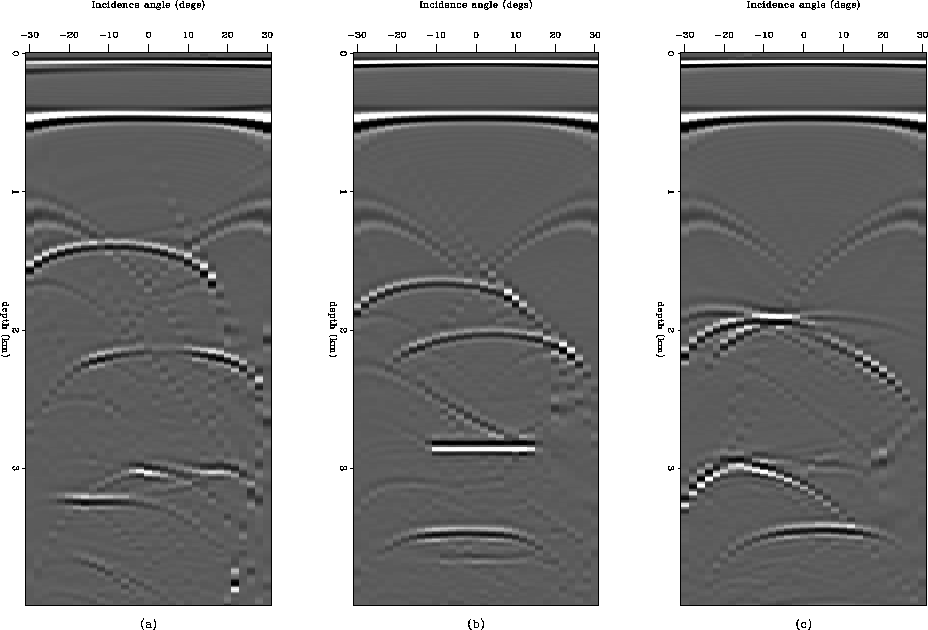
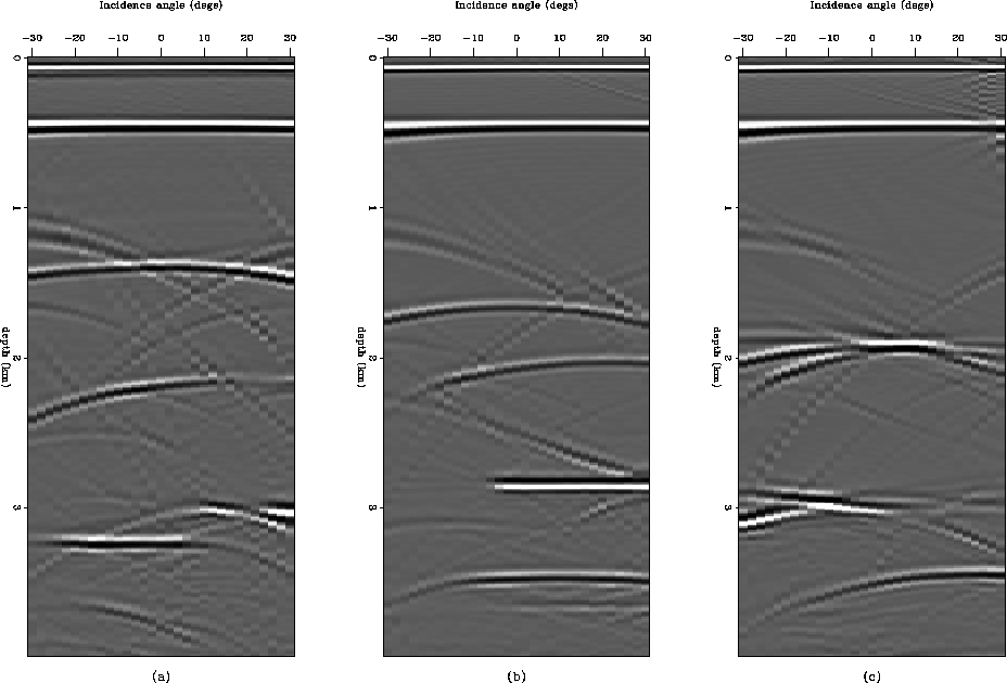
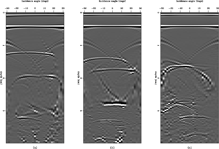
For example, I applied reflector-dependent planewave synthesis imaging for each reflector picked in the previous section (Figure pick0). Figures crp-iter0-1 to crp-iter0-4 show some of the resulting CSL gathers. In contrast to the CSL gathers obtained from surface-oriented imaging, each reflector image in the corresponding reflector-oriented imaging shows a symmetric RMO pattern with respect to the normal incidence angle. And the target images are spread all over the range of the angle used in synthesizing with equal amount of of energy, which helps to produce high amplitude in semblance stacks.

To quantify the residual moveout shown in the reflector-oriented imaging, we can use the accurate dip-dependent RMO equation derived by Zhang . However, the residual moveout equation is derived under the assumption that the medium above the reflector has constant velocity and the ray trajectories are straight lines which is not true when we deal with a variable-velocity medium. Therefore, for convenience of velocity analysis, I derived a simplified RMO equation for dipping event that resembles to the RMO equation for a flat reflector.

 

crps-iter0
Figure 6 Three CSL gathers at (a) 3 km, (b) 4 km, and (c) 5 km from the prestack image cube that was obtained by synthesizing plane waves at the surface.

 

crp-iter0-1
Figure 7 Three CSL gathers at (a) 3 km, (b) 4 km, and (c) 5 km from the prestack image cube that was obtained by synthesizing plane waves at reflector number 1.

 

crp-iter0-2
Figure 8 Three CSL gathers at (a) 3 km, (b) 3.5 km, and (c) 4 km from the prestack image cube that was obtained by synthesizing plane waves at reflector number 2.

 

crp-iter0-3
Figure 9 Three CSL gathers at (a) 3.5 km, (b) 4 km, and (c) 4.5 km from the prestack image cube that was obtained by synthesizing plane waves at reflector number 3.

 

crp-iter0-4
Figure 10 Three CSL gathers at (a) 3.5 km, (b) 4 km, and (c) 4.5 km from the prestack image cube that was obtained by synthesizing plane waves at reflector number 4.

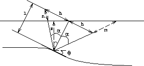
Let us consider a dipping reflector as shown in Figure crp-ray. The depth to the reflector is z, the average slowness of the medium to the reflector is $\bar w$,and t is the recorded traveltime. If a planewave source has the incidence angle $\alpha$ to the reflector, the ray path from and to the reflector will be a straight line, and the half offset h of the ray path can be approximately calculated from the incidence angle $\alpha$ of the planewave, the reflector depth z, and the dip of the reflector $\theta$, as follows :

$$h = {l \tan{\alpha}},$$ (5)

where $l = z/\cos(\theta)$ and represents the normal distance from reflector to the surface.

If we assume n=m (see Figure crp-ray), the travel time is given by

$$t = 2\sqrt{h^2+l^2} \cdot \bar w. \EQNLABEL{corr-slow}$$ (6)

After migration with the slowness of the medium, the image under a surface location will be at the same depth z. If we migrate with an average slowness $\bar w_m$instead of the slowness of the medium itself, the image under a surface location will be at depth z_m. In this case, the traveltime is given by

$$t = 2\sqrt{h^2+l_m^2}\cdot \bar w_m, \EQNLABEL{wrong-slow}$$ (7)

where $l_m = z_m/\cos(\theta)$.

 

crp-ray
Figure 11 For a reflector of dipping angle $\theta$, a plane wave satisfies Snell's law.

Note that the traveltime, t, is the same in equations corr-slow and wrong-slow because it is an observed quantity. Eliminating t from equations corr-slow and wrong-slow, we obtain

$$z_m = \sqrt{\gamma^2 z^2+(\gamma^2 -1)h^2\cos^2(\theta)}, \EQNLABEL{depth-of-gamma}$$ (8)

where

$$\gamma = {\bar w \over \bar w_m}.$$ (9)

Equation depth-of-gamma gives a relation between the apparent depth, z_m, and the actual depth, z. They are linked through the parameter $\gamma$.Note that they are equal regardless of offset or incidence angle of the planewave when the slowness used in migration is equal to the slowness of the medium ($\gamma = 1$). This is the essence of the velocity analysis principle; the image in a CLS gather is aligned horizontally if the velocity model is correct. When $\gamma$ is not equal to 1, there is both a moveout as a function of offset and a shift at zero offset.

At each depth point along the reflector, RMO is defined by the parameter $\gamma$ in equation depth-of-gamma. The data is then summed along this curved trajectory. The summation is done for a range of $\gamma$,and the sum is biggest for the value of $\gamma$that matches the curvature. Because some signals may be weaker than others, the sum is normalized. This normalized summation is similar to the normalized summation along a hyperbola using the NMO equation, commonly known as semblance (). If the data in a CSL gather is $p(z_m,\alpha)$,then searching for curvature produces the semblance panel $g(z_m,\gamma)$, defined as

$$g(z_m,\gamma) = {[ \sum_\alpha p( z=\sqrt{z_m^2 + (\gamma^2-... ...-1)h(\alpha)^2 \cos^2\theta },\alpha)]^2}. \EQNLABEL{semblance}$$ (10)

Figure velan-iter0 shows the semblance velocity analysis panel for the reflectors picked with $\gamma$ values, where the maximum semblance value for each CSL gather are on top of semblance panel. As Figure velan-iter0 shows, some of the reflectors have much lower semblance values than others. In order to avoid possible bias in inversion from this erroneous information, I excluded reflection locations that have semblance values below 0.4. The rest of the reflectors to be used in the inversion are shown in Figure npick0.

 

velan-iter0
Figure 12 Semblance stack panels for the picked reflectors. The $\gamma$ values that correspond to the maximum semblance value are overlaid on top of it with lines.

 

npick0
Figure 13 The portions of the picked reflectors to be used for determining traveltime error. The reflector locations that have below .4 in semblance value were excluded in traveltime error calculation.

From $\gamma$ to $\Delta {\bf t}$

The residual moveout velocity analysis, measuring $\gamma$,described in the previous section is just a way of measuring traveltime errors $\Delta {\bf t}$.The traveltime errors $\Delta {\bf t}$ are required to compute the perturbation $\Delta {\bf w}$ in reference slowness as shown in equation tomo-frd-linear.

The traveltime errors are the differences between the observed traveltimes ${\bf t_m}$ and the computed traveltimes ${\bf t}$ using an assumed slowness model

$$\Delta {\bf t} = {\bf t} - {\bf t_m}.$$ (11)

Both ${\bf t}$ and ${\bf t_m}$ are obtained by integrating slowness along the ray path traced through the assumed reference model,

$$\Delta {\bf t} = L ({\bf w} - {\bf w_m}),$$ (12)

and this is equivalent to an integration average slowness as follows:

$$\Delta {\bf t} = L (\bar{\bf w} - \bar{\bf w}_m). \EQNLABEL{dt-from-avgvel}$$ (13)

where $\bar{\bf w}$ and $\bar{\bf w}_m$ represent average slownesses of the true model and of the reference model, respectively.

By substituting $\bar{\bf w}=\gamma\bar{\bf w}_m$into equation dt-from-avgvel, we get

$$\Delta {\bf t} = L ( \gamma - 1 ) \bar{\bf w}_m.$$ (14)

CALCULATING THE SLOWNESS ERROR $\Delta {\bf w}$

Calculation of the slowness error $\Delta {\bf w}$by inverting the traveltime error $\Delta {\bf t}$requires first finding the back projection operator. This operator is found by ray tracing through the reference model.

A system of ray tracing equations

The ray tracing method I have implemented is based on the ray tracing system of first-order partial-differential equations, derived from the Eikonal equation by the method of characteristics ( see Cerveny for more details):

$$\begin{eqnarray} {dx_i \over ds } & = & {p_i \over w} \nonumber \\ {dp_i \over ds } & = & {\partial w \over \partial x_i } \EQNLABEL{ray-system}\end{eqnarray}$$ (15)

Here w is the slowness, x_i=x_i(s) (i=1,2,3) are the coordinates of the ray as a function of s, the arclength along the ray, and p_i(s) are the components of the slowness vector ${\bf \bar p}$.The traveltime t(s) along the ray is given by

$${dt \over ds } = w. \EQNLABEL{dtods-eqn}$$ (16)

The slowness vector is perpendicular to the wavefront (${\bf \bar p} = \nabla t$), and must satisfy

$$\vert{\bf \bar p}\vert^2 = \sum^3_{i=3}p_i^2 = w^2.$$ (17)

The system of ray equations together with equation  dtods-eqn can be solved by a standard numerical integration method. I use a fourth-order Rungge-Kutta method. It propagates the properties of the ray (x_i,p_i, and t) over an increment in arclength by combining the information from several Euler-style steps (each involving one evaluation of the right-hand side of equations ray-system and dtods-eqn), and then uses the information obtained to match a fourth-order Taylor series expansion of the ray variables at the current position.

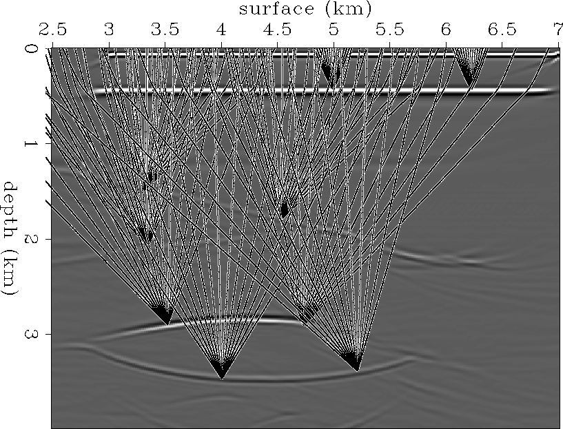
For computational efficiency, a fan of rays is traced at the same time to vectorize the code as van Trier suggested. Figure ray0 shows some of rays traced through the reference model shown in Figure synvel-iter0.

 

ray0
Figure 14 Some of the ray trajectories traced through the reference medium to calculate the operator L.

Model parameterization by spline

An accurate estimation of the gradient of the slowness field is necessary to trace rays in a velocity model with high velocity contrast. Therefore I have chosen to use cubic B-splines () to parametrize the slowness model, which enables me to calculate the slowness gradient at an arbitrary point in the model. Another reason for using splines is that a wide variety of slowness models can be represented by a few spline coefficients. This means that the number of parameters in an optimization scheme that inverts for slowness can be reduced considerably.

The spline representation of a two-dimensional slowness model is

$$w (x_1,x_2) = \sum^N_{i=1} \sum^M_{j=1} c_{ij} F_i(x_1)G_j(x_2), \EQNLABEL{spline-frd}$$ (18)

with N and M the number of spline knots in the x₁- and x₂-direction. F_i and G_j are the spline functions at the ith knot in the x₁-direction and the jth knot in the x₂-direction, respectively.

Inversion using the conjugate gradient method

After tracing rays and representing the slowness field with spline coefficients, the object function we want to minimize in the least squares sense is

$$J = ( \Delta {\bf t} - LS{\bf c}), \EQNLABEL{tomo-obj}$$ (19)

where S is the spline function shown in spline-frd, and ${\bf c}$ is a vector of spline coefficients. I used the conjugate gradient algorithm to solve the least squares problem  tomo-obj. In using this algorithm, we don't need to construct the operator L in a matrix form, which is generally huge in size. Since summing slowness along the ray paths is the forward operation and putting the traveltime error along the ray paths is the adjoint of it, we only need to store the ray paths that correspond to nonzero components of the operator L.

After finding ${\bf c}$ for the measured traveltime error $\Delta {\bf t}$, the slowness error $\Delta {\bf w}$ is obtained from spline-frd. Figure synvel-iter1 shows the slowness field updated by the least-squares inversion of $\Delta {\bf w}$.Comparing it to the true velocity model Figure synvel-iter0, we can see that the low-frequency component of the slowness field was found very well even in one iteration.

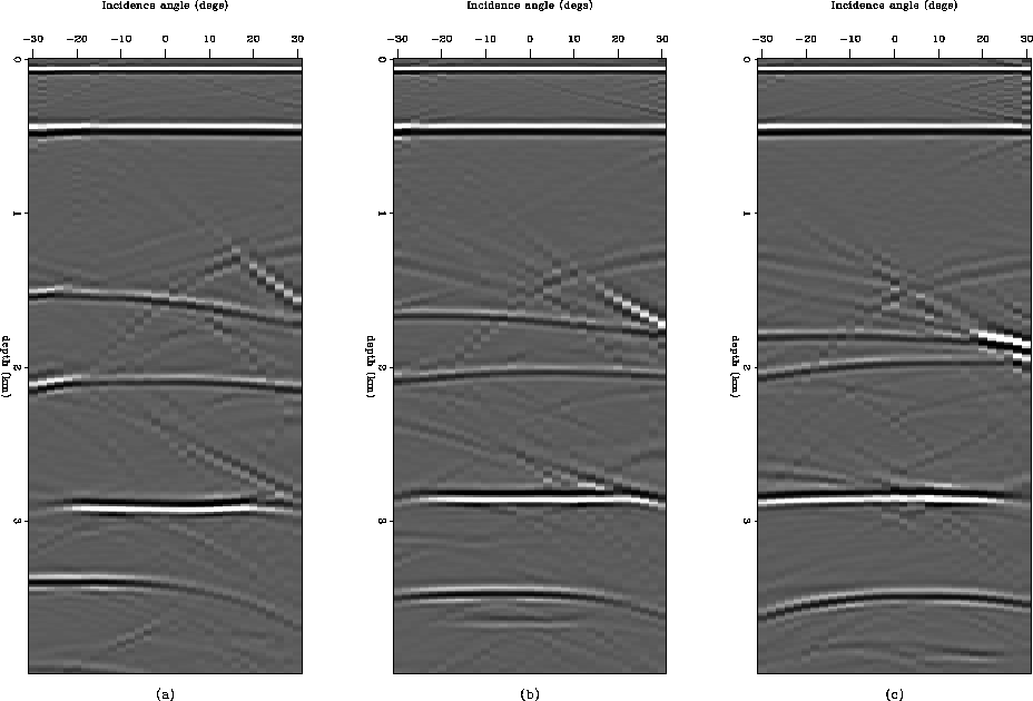
Figure pws-syn-iter1 is a stacked image after planewave synthesis imaging that synthesized 31 different incidence angles, from -30 to +30 degrees, at the surface, using the updated slowness model (Figure synvel-iter1). Most of the reflectors are located closer to the real position than that of the images obtained using the initial reference model. And CSL gathers (Figure crps-iter1) show that most of the reflectors are pretty much lined up horizontally.

 

synvel-iter1
Figure 15 Velocity model updated by adding $\Delta w$, which was calculated by inverting $\Delta t$, to the initial guess w. This corresponds to one iteration of the traveltime tomography inversion.

 

pws-syn-iter1
Figure 16 Stacked image after planewave synthesis imaging that synthesized 31 different incidence angles, from -30 to +30 degrees, at the surface. For imaging, the updated velocity model (Figure synvel-iter1) was used.

 

crps-iter1
Figure 17 Three CSL gathers at (a) 3 km, (b) 4 km, and (c) 5 km from the prestack image cube that was obtained by synthesizing plane waves at the surface using the updated velocity model (Figure synvel-iter1).

SUMMARY OF THE ALGORITHM

The tomographic velocity analysis method with planewave synthesis imaging presented in this paper can be summarized as follows:

• Define an initial model w.
• Begin Loop

  1.

  Event picking:

  • Perform surface-oriented planewave synthesis imaging.
  • Pick dominant reflectors in the stacked image.

  2.

  Measuring the traveltime error:

  • Perform reflector-oriented planewave synthesis imaging for each reflector.
  • Do RMO velocity analysis for each reflector picked.
  • Select $\gamma$ based on semblance value.
  • Convert $\gamma$ to $\Delta t$.

  3.

  Calculating the slowness error from the traveltime error:

  • Calculate $\Delta w$ by inverting $\Delta t$ using conjugate gradient.
  • Update $w = w + \Delta w$.

  4.

  Convergence test: If $\Delta w$ is small, exit from the loop.

• END Loop

This paper introduces a tomographic velocity analysis method that uses planewave synthesis imaging. In order to measure traveltime error in the image domain after prestack migration, residual moveout (RMO) velocity analysis is performed in common surface location (CSL) gathers after reflector-dependent planewave synthesis imaging. Since the reflector-dependent planewave synthesis imaging provides symmetric RMO with respect to the normal incidence angle to the reflector, the measured RMO velocity contains more accurate traveltime error information than the one of surface-oriented planewave synthesis imaging. The measured traveltime errors are inverted to determine the errors in the reference slowness in terms of spline parameters, using the conjugate gradient algorithm. The test of the algorithm for a synthetic data set shows fast convergence to true slowness model even in one iteration.

ACKNOWLEDGMENT

I would like to thank Bob Clapp for developing a convenient event-picking interface in AVS.

[my]