Amplitude-preserved low velocity noise suppression

Hector Urdaneta

hector@sep.stanford.edu

ABSTRACT

Low velocity noise can contaminate reflections and distort AVO amplitude information. I explore different inversion methods for suppressing low velocity noise while simultaneously preserving amplitudes along reflections. A velocity-stack inversion process is used for recreating models in velocity space that can reconstruct the reflections and the low velocity noise. Velocity-stack inversion is the process of creating a velocity space model that can correctly reconstruct the measured data. This is usually implemented by minimizing the L₂ norm of the data misfit and the L₂ norm of the model. Better velocity space images, with a better separation of the reflections and the low velocity noise, can be created by minimizing a different norm of the data misfit and a different norm of the model length. Norms closer to the L₁ norm appear to be better at rejecting impulsive noise and creating a spiky model. Current tests with the CORPOVEN 3-component dataset show very encouraging results.

Low velocity noise such as ground roll and air-waves contaminate reflection land data and distort AVO amplitude information. Many low velocity noise suppression techniques focus on the kinematics, e.g., predictive deconvolution or f-k filtering, without necessarily preserving amplitude information. Recently, the general increase in use of amplitudes in applications such as AVO analysis has increased the need for amplitude-preserved low velocity noise and multiple suppression ().

 

intro
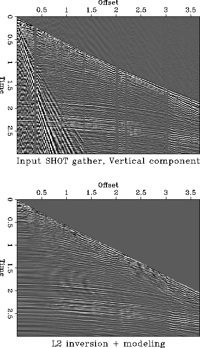
Figure 1 Top: Field shot gather from the CORPOVEN 3-component dataset (Ata et al., 1994). Bottom: reconstructed shot gather after suppression of low velocity noise, product of an L₂ velocity-stack inversion of the field shot gather, muting of the low velocity noise in velocity-stack space, and remodeling of the signal. Finally a linear outer mute of 1.8 km/s has been applied to the gather.

The top frame of Figure intro defines the problem. It shows a shot gather in which the events of interest are contaminated with low velocity noise at low offsets, distorting the AVO amplitude information. The bottom frame of Figure intro illustrates the solution I am looking for, that is, the ability to separate the interference between the noise and the the events of interest (from here on called ``the signal'') without affecting the AVO information.

With this goal in mind, I began by looking for an operator whose range has axes of time and offset, whose domain's representation of the signal and noise can be best separated, and which has an efficient and stable inverse.

Two schemes for suppressing the low velocity noise are available. The first is modeling of the signal and the second modeling of the noise. The motivation for modeling the signal is to get the best representation of the signal and to mute the noise in the operator's domain in order to reconstruct only the signal. The reason for modeling the noise is that by doing so I mute the signal in the operator's domain to reconstruct only the noise, and then subtract it from the data in order to obtain the signal. In modeling the signal there is a risk that any part of the signal that is not correctly reconstructed may artificially distort the amplitudes, which will disturb the AVO analysis. Nevertheless, modeling the signal proves to be easier than modeling correctly the noise because of the spatial aliasing of the noise.

Two processing operators are candidates for carrying out these two schemes: velocity-stack, for modeling the signal, and slant-stack, for modeling the noise. The advantage of using these two processing operators, in contrast to using physical operators, is that we are completely free to modify them to optimize our processing goal, since they have no constitutive relations that they need to satisfy. In this case it may be useful to modify the operators to make them more easily invertible (), to accelerate convergence (), or to modify the inversion norm to obtain spiky models ().

The velocity-stack operator has the disadvantage of not having an analytic inverse or a simple inverse. However, it is possible to implement the inverse transform using an iterative solver. Usually, the inverse transform is implemented as the minimization of a least-squares problem. The least-squares solution has some attributes that may be undesirable. In this paper I show the use of other types of norms in suppressing low velocity noise, following Nichols' steps for suppressing multiples. I explore the use of slant-stack inversion for modeling the noise on a synthetic example, and the use of velocity-stack inversion for modeling the signal on both a synthetic and a real example.

MODELING THE SIGNAL

As discussed above, the modeling of the signal is done with a velocity-stack operator because of the hyperbolic nature of the reflector in the gathers offset vs. time space, which produces a localized model representation of the signal in the velocity-stack space. Stacking operators are processing tools that may map data to an unphysical domain that happens to be convenient for processing reasons. The normal gather domain has axes of time and offset. The stack domain has axes of zero-offset time and velocity or slowness. Although the stacking space is unphysical, and these operators can not be derived from constitutive relations of physics, they are convenient since many data processing applications are much simpler in the stacking domain. For example, the low velocity noise may be isolated and muted in velocity-stack space, allowing reflections to be enhanced in the processed version of the input seismic data.

In doing velocity-stack inversion the aim is to create a model in the velocity-stack space in which the signal energy and the noise energy are well separated. In addition, the reconstructed data must be a good match to the signal-only part of the original data. In this section I explore modeling the signal using a velocity-stack operator. I first try using an L₂ inversion and then other inversion norms that produce more pleasing results. As an example, I use a synthetic gather that depicts some of the events seen in any of the vertical component shot gathers of the CORPOVEN 3-component dataset.

Least squares inversion

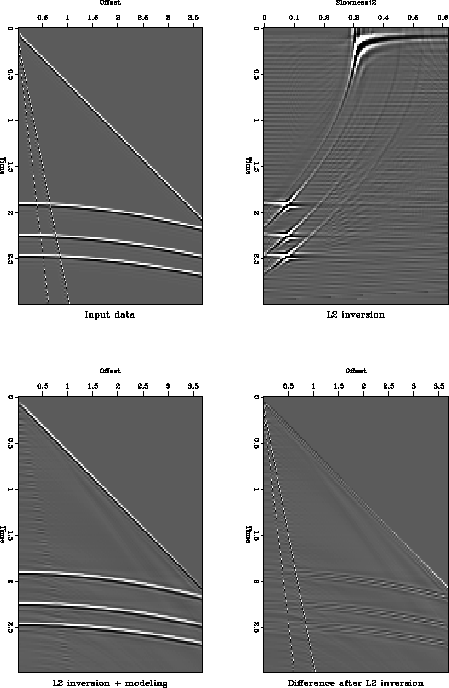
Figure L2synth displays four stages in the processing of a synthetic gather. The first frame is the original data, ${\bf d}$,consisting of three hyperbolic events, direct arrival, and two aliased events that depict the arrival of very low velocity surface waves. The second frame is its L₂ velocity-stack inverse, the third frame is the data remodeled from the inverse, and the final frame is the difference between the input synthetic and the remodeled data. The hyperbolic events of the original data are contaminated by the low velocity noise at low offsets.

 

L2synth
Figure 2 L₂ inverse processing. Top left: input data. Top right: velocity-stack inverse using an L₂ norm of the data misfit. Bottom left: reconstructed input data. Bottom right: residual data not modeled.

 

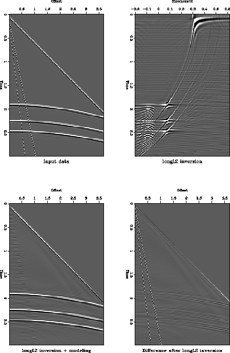
longL2synth
Figure 3 L₂ inverse processing using a wider-slowness squared range to include negative values. Top left: input data. Top right: velocity-stack inverse using an L₂ norm of the data misfit. Bottom left: reconstructed input data. Bottom right: residual data not modeled.

In the second frame of Figure L2synth I have solved the inverse problem to

$${\bf d} = {\bf V}{\bf m}$$

where ${\bf m}$ is the velocity-stack space model and ${\bf V}$ is the forward operator that maps from velocity-stack space to offset space. For the inverse problem I seek a solution to the problem of finding the model in velocity-stack space, ${\bf m}$, given the data, ${\bf d}$. This is usually posed as a least-squares minimization problem that minimizes the energy of the misfit between the modeled and measured data:

$$\min_{{\bf m}} \Vert {\bf d} - {\bf V} {\bf m} \Vert _{2}$$

The use of a conjugate gradient method in performing the inversion will not only minimize the data misfit but will also minimize the energy of the solution:

$$\Vert {\bf m} \Vert _{2}$$

Figure L2synth shows the result of the L₂ minimization of the data misfit's norm. By limiting the domain of the velocity-stack operator to low-slowness squared values and excluding the corresponding high slowness representation in the velocity-stack space of the low velocity noise, I am able to suppress the noise. Because I do not define sufficiently well where the energy of the signal lies in the the velocity-stack space, I am not able to model the signal at large offsets correctly, since we see some smearing of the signal in the residual part of the data not modeled. Moreover, we see that the noise is not completely removed.

In Figure longL2synth I have extended the domain of the velocity-stack operator to include negative-squared slownesses, which model positive curvature hyperbolas. This models the signal at large offsets more successfully, but does not yield a perfect result. Adding negative-squared slownesses to the velocity-stack domain is only possible because velocity-stack is a processing operator; it does not need to satisfy any physical laws.

Weighting the residual

We can also choose to minimize the L_p norm of the residual by minimizing the weighted residual

$$\min_{{\bf m}} \Vert {\bf W_L} {\bf d} - {\bf W_L} {\bf V} {\bf m} \Vert _{2}$$

where ${\bf W_L}$ is a diagonal operator whose i^th component is a function of the residual vector

$${\bf W_L}_{ii} = \vert r_i \vert^{(p-2)/2}$$

This is equivalent to solving the weighted problem

$${\bf W_L} {\bf V} {\bf m} = {\bf W_L} {\bf d}$$

This scheme minimizes the L_p norm of the data misfit and the L₂ norm of the model space

$$\min_{{\bf m}} \Vert {\bf d} - {\bf V} {\bf m} \Vert _{p}$$

and

$$\Vert {\bf m} \Vert _{2}$$

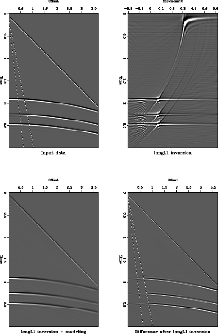
Figure longL1synth shows the result of using an L_1.1 norm to do minimize the data misfit. We see that the model is less noisy, yet the model representation of the three hyperbolic events are spread outside the domain of the velocity-stack operator. This results in a sharper image of the modeled signal, but there is a higher loss of the signal as we go to further offsets.

 

longL1synth
Figure 4 L_1.1 inverse processing. Top left: input data. Top right: velocity-stack inverse using an L_1.1 norm of the data misfit. Bottom left: reconstructed input data. Bottom right: residual data not modeled.

Weighting the model

By combining model space weights and data space weights we can minimize the L_p norm of both the data misfit and the model space. In order to do this I solve the problem

$${\bf W_L} {\bf V} {\bf W_R} {\bf \hat{m}} = {\bf W_L} {\bf d}$$

followed by

$${\bf m} = {\bf W_R} {\bf \hat{m}}$$

where ${\bf W_R}$ is the diagonal operator whose i^th component is

$${\bf W_R}_{ii} = \vert m_{i} \vert^{(2-p)/2}$$

This scheme minimizes the L_p norm in both the data misfit and the model space:

$$\min_{{\bf m}} \Vert {\bf d} - {\bf V} {\bf m} \Vert _{p}$$

and

$$\Vert {\bf m} \Vert _{p}$$

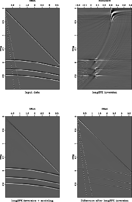
Figure longSPKsynth shows the result of using an L_1.5 norm in both domains. We see how I get a spiky velocity-stack model of the signal, which reconstructs a nicer signal, but there is some loss of signal energy at far offsets. It is encouraging that the noise has been totally removed from the reconstructed data.

 

longSPKsynth
Figure 5 Spiking inverse processing. Top left: input data. Top right: velocity-stack inverse using an L_1.5 norm of the data misfit and L_1.5 norm of model length. Bottom left: reconstructed input data. Bottom right: residual data not modeled.

MODELING THE NOISE

Modeling the low velocity noise is done using a slant-stack operator, which produces a localized noise representation in the slant-stack velocity space, because of its linear nature in the gather offset vs. time space. The goal of modeling the noise is that if I model it well, I can subtract it from the input data and obtain the signal without worrying about distorting the signal's amplitude. The aim of the slant-stack inversion is to separate as best as possible the model representations of the signal and noise.

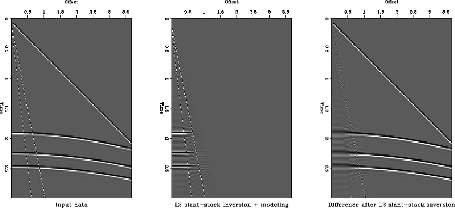
Figure ss1diff.L2 shows the result of using an L₂ norm for inverting the problem

$${\bf d} = {\bf S}{\bf m}$$

where ${\bf m}$ is the slant-stack space model and ${\bf S}$ is the forward operator that maps from slant-stack space to offset space. Just as in the inverse problem for modeling the signal, I seek a solution to the problem of finding the model in slant-stack space, ${\bf m}$, given the data, ${\bf d}$.

The middle frame of Figure ss1diff.L2 shows the reconstructed data from the slant-stack space model (not shown) and the right frame shows the data not reconstructed. We see that I am only able to reconstruct the unaliased energy of the noise while the aliased energy still contaminates the signal, so I have not succeeded in removing the low velocity noise. Even worse we notice how part of the signal gets modeled at low offsets; this is due to applying the stacking operator along the offset axis as is conventionally done.

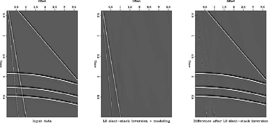
To prove this last statement, I have done the stacking along the time axis, which eliminated completely the reconstructed signal at low offsets as illustrated in Figure ss2diff.L2. Moreover I have dealiased the low velocity noise to show that to a very good extent, I have been able to suppress the low velocity noise from the data without distortion along the amplitude of the signal.

 

ss1diff.L2
Figure 6 L₂ slant-stack L₂ inverse processing. Stacking done along offset axis. Left: input data, low velocity noise is aliased. Middle: reconstructed input data. Right: residual data not modeled.

 

ss2diff.L2
Figure 7 L₂ slant-stack L₂ inverse processing. Stacking done along time axis. Left: input data, low velocity noise is unaliased. Middle: reconstructed input data (suppressed low velocity noise). Right: residual data not modeled (amplitude-preserve signal).

REAL DATA EXAMPLE

Figures ss1diff.L2 and ss2diff.L2 have illustrated the point made in the introduction that even though it is more desirable to model the noise, this is only true to the extent that we can dealias the noise. Since I do not have the right tool to dealias the low velocity noise, in the following real data examples, I have chosen to model the signal as a means of suppressing the low velocity noise.

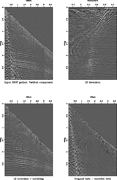
The following figures show the effect of using the various inversion methods on a shot gather from the 3-component dataset provided by CORPOVEN. () Figure real2p.L2 displays the four stages in the processing of a vertical component shot gather. The first frame is the raw shot gather, the second frame is its L₂ velocity-stack inverse, the third frame is the signal reconstructed from the inverse, and the fourth frame is the difference between the raw shot gather and the reconstructed data. I chose to process the raw data in shot gather space instead of CMP space, since in CMP space the spatial aliasing of the low velocity noise will be even greater as a result of the bigger spacing between traces in CMP space.

The CORPOVEN shot gathers are sampled at 2 msec intervals with a 6 second record length. The number of receivers per shot is 216, with a geophone group interval of 17 meters. The most relevant events occur at about 1.9, 2.1, and 2.2 seconds. The data is very rich in low velocity noise, but because it has a distinct RMS-stacking velocity from the signal, the muting of the noise in the velocity-stack space does an excelent job of removing it from the reconstructed signal, as we see from the third and fourth frames in Figure real2p.L2. There is some energy loss of the signal at far offsets, as we can see (if we look at the plot at an angle) in the fourth frame at around 2.5 kms.

 

real2p.L2
Figure 8 L₂ inverse processing. Top left: input shot gather, vertical component. Top right: velocity-stack inverse using an L₂ norm of the data misfit and negative squared slownesses. Bottom left: reconstructed input data. Bottom right: residual data not modeled.

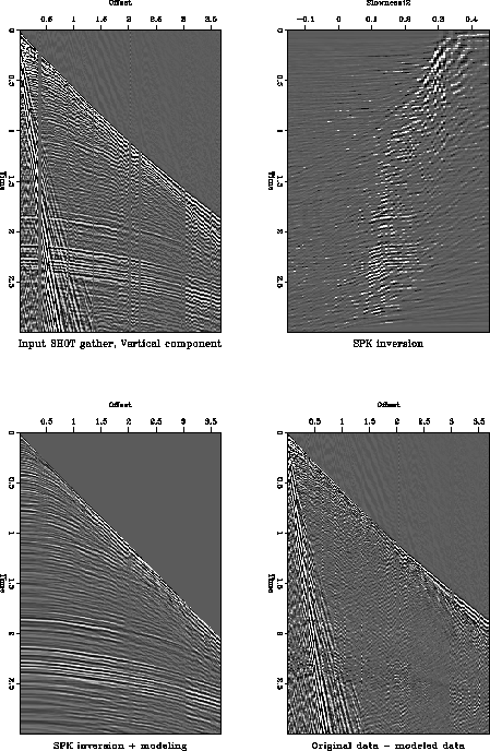
Figure real2p.SPK displays the effect of spiking inversion in the model space. The inversion minimized the L_1.1 norm of the data misfit and the L_1.1 norm of the model. The events in velocity-stack space are much more compact. This is a very desirable result, since I now obtain a better reconstruction of the signal, while suppressing completely the low velocity noise from the reconstructed data.

 

real2p.SPK
Figure 9 Spiking inverse processing. Top left: input shot gather, vertical component. Top right: velocity-stack inverse using an L_1.1 norm of the data misfit and L_1.1 norm of model length. Bottom left: reconstructed input data. Bottom right: residual data not modeled.

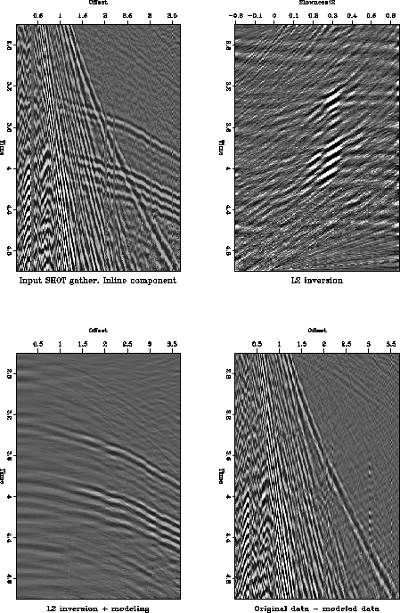
Figure real2v.L2 shows the same four processing stages of the shot gather's inline component. The first frame shows a windowed section of the gather, which is heavily contaminated with low velocity noise. It is interesting to note the dispersion of the ground roll. The higher frequencies (which are aliased), arrived first, while the lower frequencies (which are unaliased), arrived later. The second frame is the L₂ velocity-stack inverse and the third and fourth frames are the reconstructed data and the difference between the raw data and the reconstructed data, respectively. Even though the amplitudes reconstructed at near offsets are somewhat questionable, since the noise level at near offsets is so high that it completely masks away the signal, the inversion does a good job reconstructing the signal at mid and far-offsets. Looking at the reconstructed data at an angle, we can see that the reconstructed reflections at low offsets are more evident.

Figure real2v.SPK shows the use of a spiking inversion of the gather's inline component to suppress the low velocity noise, which produces a more spiky velocity-stack model.

 

real2v.L2
Figure 10 L₂ inverse processing. Top left: input windowed shot-gather, inline component. Top right: velocity-stack inverse using an L₂ norm of the data misfit and and negative squared slownesses. Bottom left: reconstructed input data. Bottom right: residual data not modeled.

 

real2v.SPK
Figure 11 Spiking inverse processing. Top left: input windowed shot-gather, inline component. Top right: velocity-stack inverse using an L_1.1 norm of the data misfit and L_1.1 norm of model length. Bottom left: reconstructed input data. Bottom right: residual data not modeled.

I have discussed two methodologies for suppressing low velocity noise while preserving signal amplitudes. The techniques involved the use of different minimization norms for the data misfit and the model length. Velocity-stack inversion is used to reconstruct the signal, and slant-stack inversion is used to reconstruct the noise. The complete liberty to modify these processing operators and the use of norms closer to L₁ produce more desirable velocity space images, with a better separation of the signal energy and the low velocity noise energy. For the real data examples, forward modeling of the velocity-stack space images produce an amplitude-preserved low velocity noise suppression. Current tests with the CORPOVEN 3-component dataset appear very encouraging.

ACKNOWLEDGMENTS

Thanks to Eulogio DelPino of CORPOVEN and Reinaldo Michelena and Manuel Gonzáles of Intevep for providing me with the CORPOVEN multicomponent dataset. I am grateful to David Lumley and Biondo Biondi for the many productive discussions about this topic. Dave Nichols' C++ solvers and operators developed for suppressing multiples were easily modified and used for suppressing the low velocity noise. Vive le C++!

[SEP,SEGCON,GEOTLE,SEGBKS,MISC,hector]