AVO estimation using surface-related multiple prediction

Stewart A. Levin

salevin@dal.mobil.com

ABSTRACT

In this work I explore the use of surface multiple prediction in enhancing AVO estimation. Multiple reflections from a proposed reflection event are predicted using surface-related multiple prediction () and compared to the actual data to identify anomalous amplitude behavior.

 Surface-related multiple attenuation is derived from a surface-related multiple feedback equation

U = (1-U) R

which expresses the fact the the recorded data U is the sum of the direct illumination of the subsurface R and the secondary illumination with the reflected data -U. (A more precise formulation is given by Wang and Levin .) In particular, the surface multiples in our data are given by the term -UR. Each primary reflection, P, in R produces the multiple train -UP.

Suppose we now generate a synthetic primary reflection, P₀, with constant amplitude that matches the moveout of an actual event in our data. Assuming our data is relative amplitude compensated (i.e. divergence corrections and cable balancing are applied), then the AVO response of the multiple prediction -U P₀ should match the AVO of the multiples in the actual data just as the AVO response of the primary P₀ should match the AVO of the actual primary it models. If there are systematic deviations, we conclude that we are seeing an AVO effect.

This strategy offers some potentially nice features:

• It is an incremental improvement to conventional AVO. The additional information given by multiples may enhance and stabilize AVO estimation from multiple-contaminated data.
• The approach relies only on relative amplitudes along events. The absolute scaling may change from one arrival to another. Unlike multiple attenuation, I do not seek to match absolute amplitudes.
• Since multiple reflections amplify small time differences, a later multiple may separate from a strong interfering event, allowing AVO estimation to proceed unhampered.
• Because the angular aperture of later arrivals is smaller, the angular resolution of AVO measurements from multiple reflections is higher.

1-D The surface multiple prediction works on prestack data from a 2-D line. In the special case of a horizontally-layered earth, the process reduces to a 2-D convolution of a representative shot record with the proposed primary event. This is equivalent to multiplying their $\omega$-k_x transforms together, making investigation of the process exceptionally easy without losing the generality of the full prestack prediction.

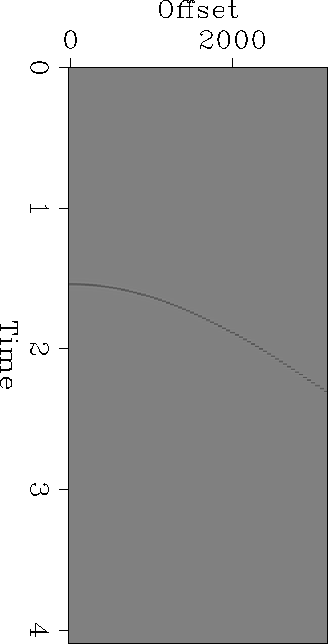
Let us look at a synthetic example. Figure gather1 is an elastic synthetic seismogram generated for a point source over a 1-D earth model. This model was developed from well logs provided with the Mobil AVO dataset. Using the interactive Overlay program (), I picked the seafloor reflector and generated a flat, constant-amplitude event with the same zero-offset intercept. Filtering to the frequency range of the synthetic and inverse NMO application produced the template in Figure waterbottom. Convolving these together produces the surface multiple train in Figure waterbottom-multiples. With the exception of some aliased energy and finite-aperture artifacts, the predicted multiples align well with the multiples in the data. The phase differences are due to the half derivative implicit in two-dimensional hyperbolic summation being applied to data generated in three dimensions.

 

gather1
Figure 1 Synthetic elastic seismogram generated by Haskell-Thompson modelling.

 

waterbottom
Figure 2 Constant-amplitude model of water bottom reflection.

 

waterbottom-multiples
Figure 3 Water bottom multiple train prediction by convolving the datasets in Figures gather1 and waterbottom.

CORRELATING OFFSETS

The ability to model relative amplitudes along multiple reflection events is not useful unless we can correlate the amplitude changes to specific offsets, or at least offset ranges, of the corresponding primary reflection. The way I've chosen to approach this problem is to emulate a ``beam'' by applying bell-shaped weights centered around specific offsets on the model primary. By inserting this smoothly-peaked function into the process, I generate a template of multiple arrivals associated with this offset. Figures waterbottom-near-offset and waterbottom-middle-offset show sample bell-weighted primaries and Figures waterbottom-multiples-near-offset and waterbottom-multiples-middle-offset show the corresponding multiple event templates they generate. You can clearly see the constant-slope peaks moving approximately radially. This amplifies the point made in the introduction: later arrivals have less angular aperture and more angular resolution. Furthermore, the aliasing artifacts from Figure waterbottom-multiples, which arise from the steep, aliased portion of the hyperbola in Figure waterbottom, are no longer present.

 

waterbottom-near-offset
Figure 4 Model of water bottom reflection bell-tapered around zero offset. The half-width of the taper is about 150 m.

 

waterbottom-middle-offset
Figure 5 Model of water bottom reflection bell-tapered around an offset of 750 m.

 

waterbottom-multiples-near-offset
Figure 6 Multiple template of zero-offset multiples.

 

waterbottom-multiples-middle-offset
Figure 7 Multiple template of near-offset multiples.

AVO ESTIMATION In the previous sections we have seen that multiples can be predicted and offsets can be correlated between primary and multiple arrivals. Now I turn to AVO estimation using these tools. Three strategies come to mind, which I order according to what stage the user needs to pick amplitudes:

1.

Apply a conventional AVO measurement procedure to the multiple-contaminated data and use the offset correlations to combine primary and multiple AVO.

2.

Use the multiple template to decide where to pick amplitudes and use the offset correlations to combine primary and multiple AVO.

3.

Combine the offset-restricted multiples with the input dataset, by, say, normalized cross-correlation, and pick a suitable peak as the AVO measurement.

Strategy 1 is severely hampered by the fact that multiples generally do not flatten at primary velocity, but AVO is measured along constant time slices. It will be necessary to perform velocity scans on the predicted multiples for each separate primary reflection of interest. This is essentially strategy 2 -- use the multiple template to tell us where to pick amplitudes on the multiple-contaminated data. At the time of this progress report, I have not yet worked around bugs or limitations in ProMAX that prevent me from successfully applying the needed NMO velocity profile to flatten the multiples for AVO picking.

Strategy 3 avoids direct amplitude picking and relies on being able to emulate multiples well enough so that amplitude variations with offset are not dominated by artifacts of the emulation algorithm. A fit of the offset-limited multiple panels to the input data then provides AVO estimates.

Least-squares fitting

My approach to strategy 3 is illustrated in Figures t1552-model through product-t1552-x1000. The offset axis is broken into a series of partially overlapping ranges from which a sequence of multiple models, M₁ to M_n, are generated. A least-squares problem is then set up

$$U \approx \sum_1^n a_j M_j\EQNLABEL{approxfit}$$ (2)

to estimate AVO coefficients a_j. Dividing through by the first coefficient produces an amplitude versus offset curve from the multiple template. I use a weighted least-squares approach in order to accommodate divergence, and possibly other, corrections.

 

t1552-model
Figure 8 Model of deeper reflector at 1.552 sec.

 

product-t1552-x0
Figure 9 Multiple model for zero-offset of deeper reflector.

 

product-t1552-x1000
Figure 10 Multiple model for intermediate offset of deeper reflector.

In more detail:

1.

The input data are scaled by t^1/2 to emulate 2D divergence.

2.

A primary reflection is identified with the Overlay program.

3.

A constant amplitude model is

• generated at the primary reflection time,
• bandpass filtered,
• inverse NMO'ed with the primary velocity, and
• scaled by t^-1/2 to emulate 2D divergence

to produce a primary template.

4.

the offset range is divided into approximately equal, partially-overlapping pieces.

5.

For each offset segment:

(a)

The constant amplitude model is bell-tapered for that segment. The tapers are renormalized so that they sum to 1 between the first and last bell centers.

(b)

The range-limited primary synthetic is suitably convolved with the input data to emulate multiples.

(c)

The multiple template is rho-filtered to correct for 3D-to-2D phase differences.

6.

The suite of offset-limited panels and the input data are scaled by t^1/2 as partial preconditioning.

7.

The reciprocal envelope of the input data is computed and muted to just prior to the arrival of the first multiple. These weights are used for preconditioning of the least-squares ().

8.

Not yet implemented: Each multiple panel is cross-correlated with the input data to estimate and apply a small residual alignment.

9.

A least-squares fit is done to estimate the AVO coefficients a_j in equation  .

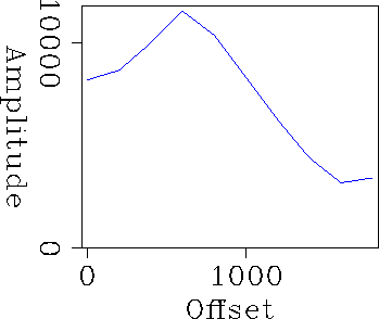
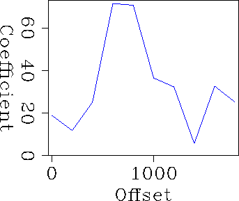
Applying this procedure to the data over the offset range 0-1800 meters, produces the AVO estimation of Figure avocoeffs. Picking the largest amplitude sample at the corresponding offsets on the primary event yields Figure primary.AVO. While we can see that both graphs have the same general trend, peaking around offset 600-800 m., the multiple estimates jump around a good deal more.

 

primary.AVO
Figure 11 Relative amplitudes picked from primary reflection.

 

avocoeffs
Figure 12 Relative amplitudes estimated from multiples.

Blinking between the multiple template and the input data shows the probable cause of the instability -- a progressive timing shift between the early and late multiples. This reflects the sensitivity of multiples to small timing differences. In this case my zero-offset intercept time looks to be about 4 ms. too large for the model primary. Future work to appear at this year's SEG AVO workshop will address this (cf. item 8 above.)

[SEP,SEGCON,MISC]