The quest for anisotropic moveout

Martin Karrenbach and Francis Muir

martin@sep.stanford.edu, francis@sep.stanford.edu

INTRODUCTION There is renewed interest in velocity anisotropy, and publications of researchers outside SEP describe various schemes for estimating anisotropic moveout from seismic data. However, those schemes often face problems in that they commit too early to a particular class of elastic models which may require auxiliary information not available from surface seismic data. In essence, they are model-driven, not data-driven. This distinction has long been understood at SEP, where there is a ten-year record of developing practical schemes for characterizing non-hyperbolic moveout, whatever its cause. In this paper we distil the anisotropic wisdom of our past and outline the key features of a practical estimation procedure. Two data examples illustrate a method for estimating and removing anelliptic moveout in a CMP gather.

THE KEY FEATURES OF A PRACTICAL SCHEME

Here are the key features of the practical estimation scheme that we are currently using and are trying to promote:

• data driven and not model driven
• one extra parameter for surface seismic (easily extendible)
• Dix-like decomposition into interval properties
• easy conversion from ray domain into wave domain and vice versa
• bombproof approximation (cannot blow up)
• estimation in time domain and then conversion into depth domain
• estimation of lithology at the end of the processing flow
• easy conversion to other processing domains
• common mathematical structure for all approximation levels

Let me now describe the above points in more detail.

The approximation is completely data driven and as such avoids the pitfalls of model driven formulations. The decision about what kind of earth model is causing the anelliptic moveout is in our case delayed until the end of the processing steps, while in model driven approaches, the model is determined from the outset and thus a specific cause of anisotropy is assumed.

The anelliptic approximation has for surface seismic data just one extra robust parameter besides the NMO velocity that has to be estimated. It completely specifies the moveout curve. More parameters can be added if necessary in order to incorporate information that is available through other experiments, such as VSP, cross hole data and well logs.

The parameters and its mathematical form are chosen such that there exists a Dix-like decomposition of the stack parameter and its associated interval parameter. It is a natural extension of Dix's formula and can be cast as an Abelian group. This makes it very easy to calculate interval properties for any of our approximations

Our approximation has a very simple way of converting from the ray domain into the wave domain and vice versa. Many other approximations have to go through a parametric relationship involving angular derivatives to convert to and from different domains. A simple Taylor expansion cannot accomplish that task. Conversion is necessary if, for example, traveltime data are observed and velocities and parameters are estimated from it. Using this information in a wave domain setting such as a wave equation downward continuation or migration requires the information to be transformed and used as dispersion relation. This is where the difference between the ray and phase velocity and anelliptic parameters becomes significant.

When estimating velocities and anelliptic parameters from moveout curves, we need to make sure that the approximations produces reasonable results bombproof in the entire range of usage. Taylor expansions have a hard time achieving this goal, while a rational polynomial is a robust contender.

We can work purely in the time domain and can easily go to the depth domain as the last processing step, where a depth mapping velocity has to be used. The main advantage, however, is that we are not forced to work in either domain, but can choose our domain. Obviously, this depends on the types of data we have available for the problem. Many other approximations will work in only one domain and thus require special information from the beginning.

After the parameter estimation is carried out, we can easily infer lithology from the estimated parameters, transverse isotropic in 2D, orthorhombic in 3D. However, we are not committed to a certain model from the onset.

The anelliptic approximations easily transform into other convenient processing spaces $p-\tau$ or p-t, etc.

The most striking feature is the common mathematical structure across all formulations; this makes for an elegant mathematical description and processing tool.

DATA EXAMPLE

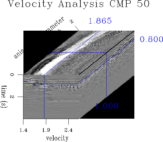
We chose a typical marine dataset to determine anelliptic moveout from surface seismic data. Figure kjarinv shows the analysis of one CMP gather out of Kjartansson's Gulf Coast dataset. A single parameter anelliptic approximation prescribes a stacking trajectory. We show a velocity inversion cube, where we iterated using the moveout-stack operator to find the optimum model representation for this CMP gather. The front panel view corresponds to the conventional velocity analysis panel, while the third axis varies the anelliptic moveout parameter. That anelliptic moveout parameter variation can be seen for a constant times slice in the top panel of the cube. The time chosen shows an event which has a slight anelliptic moveout. But this panel also shows a strong variation of the anelliptic parameter with stacking velocity. The derivation of this parameter can be found in () and is the ratio of horizontal direct velocity versus vertical NMO velocity; recently this parameter has essentially been rediscovered by other researchers, which confirms our earlier findings.

 

kjarinv
Figure 1 Stacking velocity inversion for a single CMP gather from Kjartansson's dataset. The single parameter anelliptic approximation was used to calculate the moveout stacking trajectory. The stacking operator was iterated about 10 times and sharpened the least-squares velocity analysis panel (front view) considerably.

CONCLUSION Velocity scans using the single elliptic approximations with one anelliptic parameter have been applied to a real dataset from the Gulf of Mexico. For some events the scans show clear deviation from the isotropic model. It is not clear if this is caused by intrinsic anisotropy or layering or simply by heterogeneity. Whatever mechanism produced the anelliptic moveout, the double elliptic approximation finds a way to estimate it. However, the parameter and the NMO velocity are not linearly independent and this manifests itself as smooth curves in the parameter-velocity plane of the CMP-scan volume.

[SEP,MISC]