 |
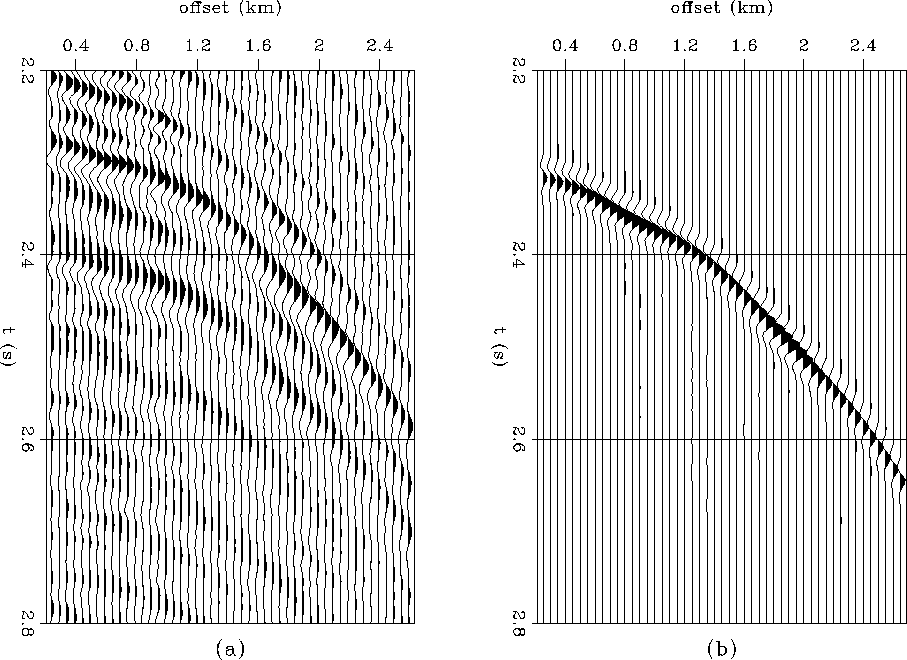
Figure 1 (a) A windowed portion of a CMP gather from the Grand Isle data set. The events have kinematic and amplitude distortions due to near-surface velocity anomalies. (b) A synthetic CMP gather with the same types of distortions.
![[*]](http://sepwww.stanford.edu/latex2html/prev_gr.gif)
ABSTRACTNear-surface velocity anomalies cause kinematic and focusing effects which can be ameliorated by wave-equation datuming and layer replacement. The trick is to find the correct datuming velocity. When the anomalies are shorter in lateral extent than the cable length, residual times picked from deep non-hyperbolic events can be used for traveltime tomography. The optimal reconstruction is obtained by constraining the model to the near surface and by estimating the inverse covariance matrix with a prediction error filter. Downward continuation with the traveltimes from this model, followed by upward continuation with a replacement velocity, removes most of the unwanted distortions. |
Seismic data are often plagued by near-surface velocity variations which adversely affect processing, imaging and interpretation. Focusing and defocusing of the wavefield as it propagates through these anomalies causes kinematic and amplitude distortions which cannot be adequately compensated by conventional static shift methods.
Kjartansson (1979) demonstrated that these types of anomalies can be detected by performing an inversion with either trace energy calculated in a time gate or with residual traveltimes calculated by crosscorrelating traces in a time gate. He chose his time gate to be substantially deeper than the location of the velocity anomalies and performed his inversion by assuming linear raypaths. This method can be implemented by performing iterative slant stacks of the trace energy or residual traveltime data in midpoint-offset coordinates (Claerbout, 1993). The resulting depth images locate the anomalies in midpoint and depth, but do not provide a method of estimating the velocity.
I use traveltime tomography to determine the near-surface velocity for datuming and layer replacement. By restricting the tomographic solution to the near surface, I can use the assumption of straight raypaths in the near surface while implicitly allowing the raypaths in the deeper part of the model to be curved. This relieves some of the constraints imposed by Kjartansson's assumption that the entire raypath is straight. Another benefit of restricting the solution to the near surface is that the problem becomes more overdetermined. I implement the tomography so that I simultaneously solve for the prediction error filter (PEF) which estimates the inverse covariance matrix (Claerbout, 1994). This last feature of the inversion brings the inverted amplitudes up to the correct values and reduces tomographic artifacts.
The method is designed to estimate near-surface velocity anomalies which are shorter in lateral extent than the cable length. A basic assumption is that the wavefield can be propagated through the near-surface to some datum below the anomalies. If the appropriate velocity is used for datuming, the effects of the anomalies are removed from the data.
I start out by reviewing the nature of problem and by describing how I generate synthetic data. I then describe the tomographic inversion and use the velocities obtained from it to generate traveltimes for Kirchhoff datuming and layer replacement.
NEAR-SURFACE VELOCITY ANOMALIES
The effect of near-surface velocity anomalies is seen in a CMP gather from Kjartansson's Grand Isle data set as non-hyperbolic moveout and amplitude variation with offset (Figure realsyna). These effects are caused by anomalies which are shorter in lateral extent than the recording cable. Figure realsynb is a synthetic shot gather generated using a Kirchhoff modeling program. I have not attempted to model the Grand Isle data exactly, but it is evident that the synthetic embodies the same non-hyperbolic moveout and amplitude variation with offset as the real data.
The effect of the amplitude variation is more evident in the moveout corrected CMP's of Figure realsynnmo. These are the same CMP locations as in Figure realsyn. The top synthetic was generated with slow near-surface velocity anomalies, the middle synthetic was generated with fast near-surface velocity anomalies. The bottom frame is the CMP gather of Figure realsyna after NMO. The slow synthetic matches the character of the data better than the fast synthetic.
 |
 |
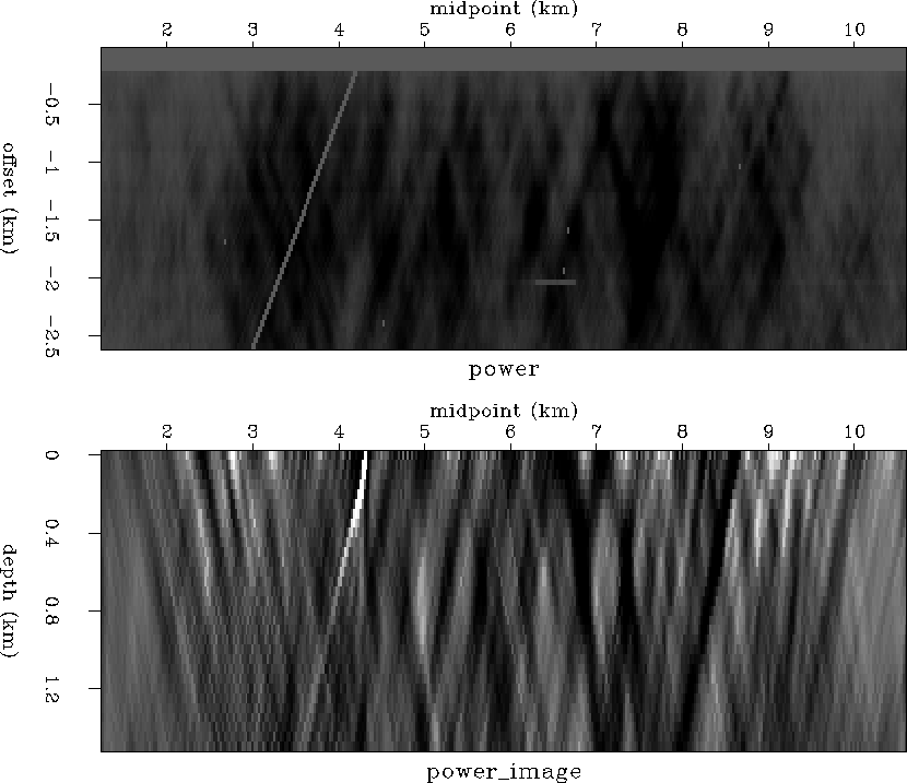
In Figure gitomo.power, I have applied Claerbout's (1993) implementation of Kjartansson style tomography. Performing iterative slant stacks of trace power in midpoint-offset coordinates has located the velocity anomalies laterally and in depth. Two prominent low velocity anomalies are located near 7 km at a depth of about 500 m. The result of performing the same type of tomography on the residual traveltime picks is presented in Figure gitomo.tpick. The traveltimes were generated by crosscorrelating the normal moveout corrected traces and picking the peak correlation amplitude. As in Kjartansson's case, the traveltime image is of poorer quality than the amplitude image.
 |
 |
Modeling near-surface anomalies
The synthetic gathers shown in Figures realsyn and realsynnmo are generated using Kirchhoff modeling and datuming codes similar to those described in previous reports (Bevc, 1993; Bevc, 1994). Finite difference traveltimes were used to calculate the necessary Green's functions for the Kirchhoff datuming algorithm (van Trier and Symes, 1991; Popovici, 1991).
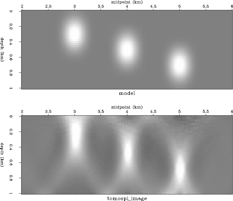
The model used to generate the synthetics consists of three near-surface velocity anomalies in a constant velocity background of 2.1 km/s (Figure model). There is a single reflector at a depth of 2.4 km and the anomalies are centered at depths of 300 m, 500 m, and 700 m.
|
model
Figure 5 The model used to generate the synthetics has a reflector at a depth of 2.4 km and three anomalies near the surface. Synthetic gathers were generated for both fast and slow near-surface anomalies in an otherwise constant velocity medium. | 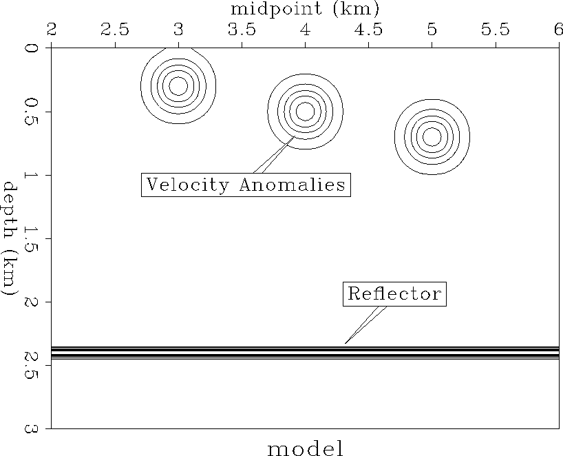 |
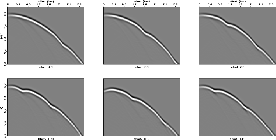
Representative synthetic shot gathers are shown for slow and fast anomalies in Figures syn.slow and syn.fast. The peak values of the velocity anomalies deviate about 15 % from the background velocity.
 |
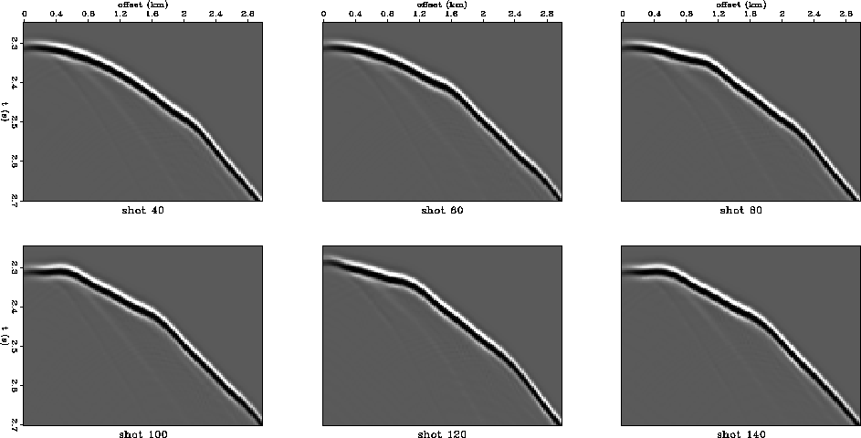 |
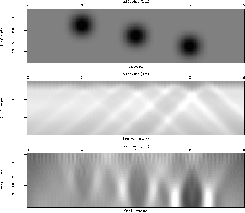
Figure kjimage.slow displays the slow velocity model, the corresponding trace amplitude plot, and the result of performing the Kjartansson style tomography. The width and amplitude of the trace power streak increases with increasing depth because the Fresnel zone increases. This has the effect of making the image of the shallowest anomaly much weaker than the other two. The image displays typical tomographic artifacts such as elongation along the depth axis and ``X'' patterns due to backprojection trajectories. The imaged anomalies are laterally smaller than the actual anomalies because a straight ray assumption is used in the inversion. Slow anomalies appear smaller because the true Fermat raypath will tend to go around the slow region; However, under the assumption of straight ray reconstruction, the residual is backprojected along a straight line so that the effects of a slow region are focused into a smaller region (e.g. Berryman, 1991).
 |
Figure kjimage.fast displays the same results for the fast near-surface velocity anomalies. The images appear larger than the actual anomalies because the backprojection of a fast anomaly with straight rays tends to spread into a larger region.
 |
The tomographic images presented in this section confirm the presence of near-surface anomalies in the data and the synthetics. The synthetics confirm that kinematic focusing can cause the amplitude anomalies observed in the Grand Isle data. Although Kjartansson's method can detect and locate anomalies, it does not provide a means of estimating the near-surface velocity. In order to do that, I have developed the constrained tomographic method of the next section.
TRAVELTIME TOMOGRAPHY Wave-equation datuming has been demonstrated to be effective for downward continuing marine data through the water layer and performing layer replacement (Yilmaz and Lucas, 1986; Berryhill, 1986). In that application, the datuming velocity is well known. In my application it is unknown. In order to find the datuming velocity, I backproject residual traveltimes picked from deep non-hyperbolic events.
The goal of the method is to improve imaging by removing distortions
from events. Except for the near-surface anomalies, the velocity
structure of the Grand Isle data is pretty simple, so that normal
moveout correction and stacking provide an adequate imaging method.
Stack power is
maximized when events have hyperbolic trajectories. This means that
after NMO correction, events should be flat.
A measure of this flatness is to crosscorrelate a
pilot trace tpilot with the data after NMO. The maximum
lag of this
crosscorrelation gives a time shift ![]() which is the residual
traveltime to be backprojected (k is a trace index).
The objective function to be minimized is then
which is the residual
traveltime to be backprojected (k is a trace index).
The objective function to be minimized is then
| (1) |
The traveltime calculation can be linearized by assuming straight rays and writing the traveltime as
| (2) |
| (3) |
| (4) |
| (5) |
If the inverse covariance matrix is unknown (as is usually the case),
it can be estimated by considering ![]() to be a prediction error
filter with coefficients to be determined (Claerbout, 1994).
The model and the prediction error filter can then be written as
to be a prediction error
filter with coefficients to be determined (Claerbout, 1994).
The model and the prediction error filter can then be written as
| (6) |
| (7) |
| (8) |
| (9) |
The data space and model space residuals are defined as:
| (10) |
| (11) |
This system of equations is solved using the method of conjugate gradients. The first step in the solution is to initialize the model by calculating
| (12) |
| (13) |
| (14) |
| (15) |
In summary, the conjugate gradient solution begins by initializing the model and filter with equations init1 and laplacian. The residuals are initialized using equation residuals and iterations begin by calculating the gradient [equation gradient] and the conjugate gradient [equation conjgradient]. In practice, the algorithm is allowed to run for a while using the Laplacian filter of equation laplacian before the prediction error filter coefficients are found.
SYNTHETIC EXAMPLES
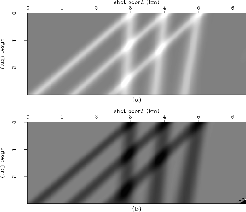
The synthetic data of Figures syn.slow and syn.fast are used to test the tomography algorithm of the previous section. Figure picktt is a plot of the residual traveltimes which represent the deviation of the curves in Figures syn.slow and syn.fast from hyperbolas. The effects of the slow anomalies are confined to narrow trajectories and the effects of the fast anomalies are spread over wider trajectories.
 |
The resulting tomograms will be used to calculate traveltimes maps for the Kirchhoff datuming code. In order to compare the tomographic results, I present the travel time map generated by calculating finite-difference traveltimes in the near-surface velocity model depicted in Figure model. Figure resid.tt.slow is a display of the residual traveltime from each subsurface location at 1 km depth (horizontal axis) to all surface locations (vertical axis). These traveltimes can be considered to be the goal of the tomographic inversion since they are the desired datuming traveltimes.
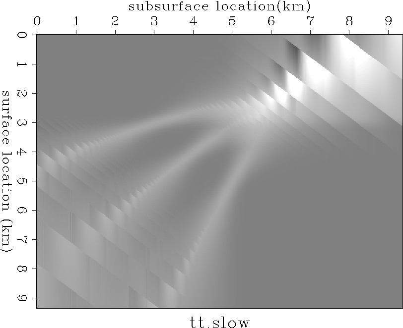 |
The tomographic image obtained with the simplest backprojection algorithm (equation regression) is compared to the original depth model in Figure tomo.tomospl.slow. Although this image is considerably better than the Kjartansson style tomogram of Figure kjimage.slow, it exhibits undesired artifacts such as vertical elongation and ``X'' patterns. This slowness image is used to calculate the finite-difference traveltime map displayed in Figure resid.tt.tomospl.slow. This map does not match the traveltime map of Figure resid.tt.slow very well.
 |
 |
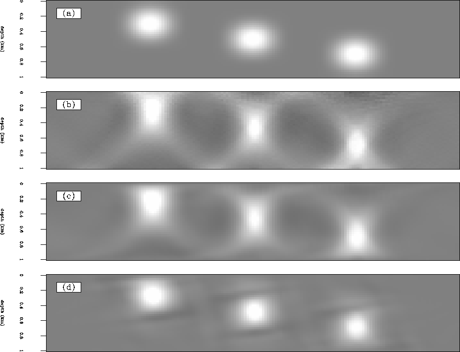
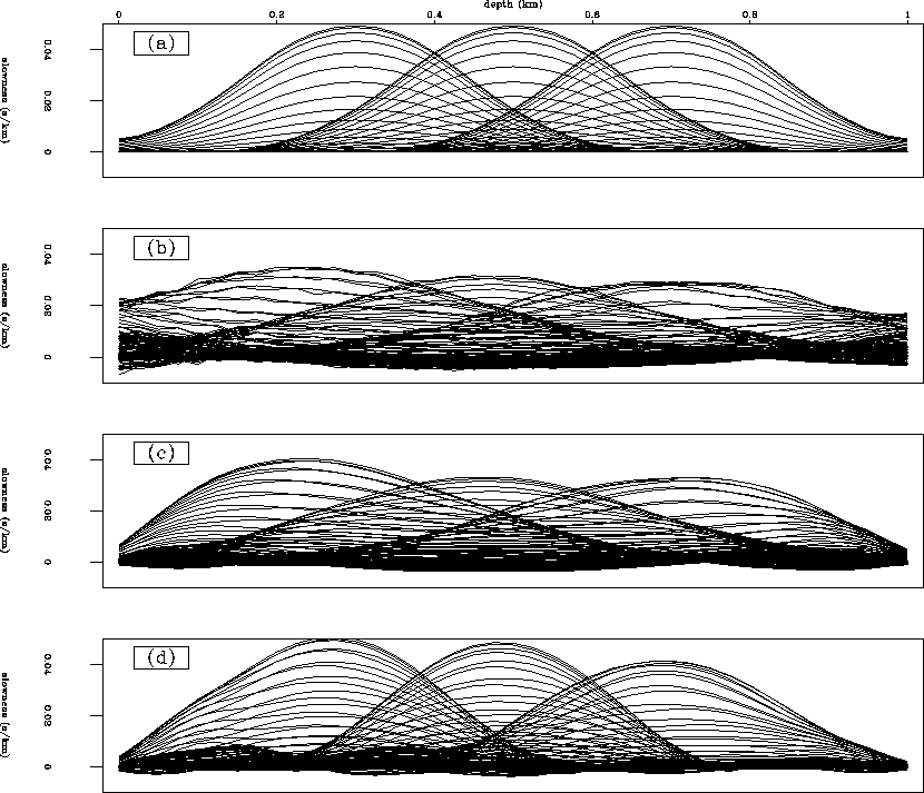
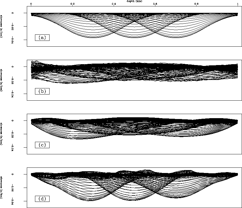
Figures comptomo.slow and comptomo.fast are a comparison of the original depth model to several tomographic images. The slow images (Figure comptomo.slowb to comptomo.slowd) look smaller than the fast images (Figure comptomo.fastb to comptomo.fastd) because the residuals are backprojected along straight lines. The amplitudes of the various tomograms are compared in Figures compamp.slow and compamp.fast.
Using the prediction error formulation of equation peftomoreg (frame c in Figures comptomo.slow through compamp.fast) is a significant improvement over the simpler formulation of equation regression. (frame b in Figures comptomo.slow through compamp.fast): The amplitudes in frame c look smoother and the images are better located. The reconstruction artifacts are also ameliorated.
By using the knowledge that straight ray reconstruction broadens fast anomalies and compresses slow anomalies, the information from the images generated by equation peftomoreg in frame c of Figures comptomo.slow through compamp.fast can be used to add additional constraints to the inversion. The result of doing this is displayed in frame d of Figures comptomo.slow through compamp.fast. These images match the original depth models (frame a of Figures comptomo.slow through compamp.fast) pretty well. The most significant improvement is in the amplitudes and in the reduction of reconstruction artifacts.
 |
 |
 |
 |
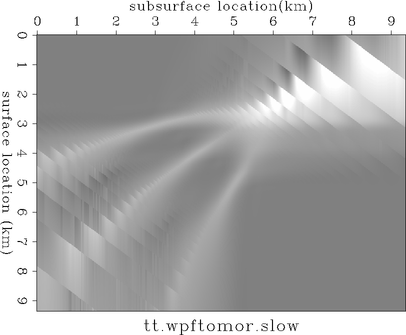
A closeup of the inversion result using the prediction error filter to estimate inverse covariance as implied by equation peftomoreg and model constraints is displayed in Figure tomo.wpftomor.slow. This is the same image as Figure comptomo.slowd. The corresponding traveltime map, shown in Figure resid.tt.wpftomor.slow, matches the desired traveltime map of Figure resid.tt.slow almost exactly.
 |
 |
LAYER REPLACEMENT
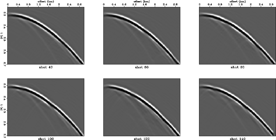
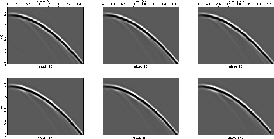
The traveltimes of Figure resid.tt.wpftomor.slow and a similar set of traveltimes for the fast near-surface anomalies are used to generate kinematic Green's functions for Kirchhoff wave-equation datuming. The result of layer replacement for the slow and fast models is shown in Figures rep.wpftomor.slow and rep.wpftomor.fast. The events now exhibit hyperbolic moveout.
 |
 |
DISCUSSION AND CONCLUSIONS
I backproject residual traveltimes picked from deep non-hyperbolic events to determine the near-surface velocity for datuming and layer replacement. The best image is obtained by constraining the solution and by solving for both the slowness and the coefficients of the prediction error filter which estimates the inverse covariance matrix. Once the near-surface velocity model is found, wave-equation datuming is used to perform layer replacement and remove unwanted distortions.
The tomographic solution may be non-unique; however, this is not a problem because the ultimate goal is to remove distortions from deeper events. So it does not matter if the velocity used for datuming is an accurate representation of the of the actual velocity. It only needs to provide an adequate representation of the kinematics. I am not interested in imaging the near surface, just in removing its deleterious effects.
The method presented here works well on synthetics. It may not work as well on real data, so a more sophisticated velocity estimation method, such as the one outlined in the Appendix, may be required.
REFERENCES
An alternative to traveltime tomography is to perform a wavefield inversion by formulating the problem in terms of maximizing a non-quadratic objective function. This formulation is more computationally intensive, but it does not require crosscorrelation and picking and may be less sensitive to noise. Similar approaches are employed by other authors for different velocity estimation settings (Toldi, 1985; Fowler, 1988; Biondi, 1990; Etgen, 1990)
Maximizing stack power In formulating the objective function, I assume that I can get a good estimate of the overall background velocity structure, minus the near-surface anomalies (i.e., approximate stacking trajectory). After wave-equation datuming with the best estimate of near-surface velocity, the stack power is maximized. Formally, this can be expressed as maximizing the following non-linear objective function:
 |
(16) |
In this formulation, the data have been downward continued from the
surface having shot and group coordinates ![]() , to
a datum below the near-surface anomalies having shot and group
coordinates (xs,xg). I express the Kirchhoff
downward continuation (without the cluttering detail of amplitude and
phase terms) as a summation over shot and group coordinates:
, to
a datum below the near-surface anomalies having shot and group
coordinates (xs,xg). I express the Kirchhoff
downward continuation (without the cluttering detail of amplitude and
phase terms) as a summation over shot and group coordinates:
| (17) |
![]() is a complicated function of traveltime and slowness.
The gradient of the objective function with respect
to the model parameters is calculated by applying the chain rule:
is a complicated function of traveltime and slowness.
The gradient of the objective function with respect
to the model parameters is calculated by applying the chain rule:
![\begin{displaymath}
\EQNLABEL{gradp}
\begin{array}
{l}
\nabla_{\hat m} Q_p \;=\;...
... t}{\partial m}(x_s,\xi_s,x_g,\xi_g)
\right)\right]\end{array}\end{displaymath}](img33.gif) |
(18) |
The nonlinear inversion implied by equation gradp then proceeds
by (1) evaluating the gradient ![]() and (2) using it
to update the slowness model
and (2) using it
to update the slowness model ![]() .The step size
.The step size ![]() is determined so that it maximizes Qp.
Iterations are continued until convergence.
is determined so that it maximizes Qp.
Iterations are continued until convergence.
Maximizing semblance Instead of maximizing stack power, which favors large amplitudes, a better alternative might be to maximize semblance,

| (19) |
The gradient of the objective function with respect to the model parameters is then
| (20) |
![[*]](http://sepwww.stanford.edu/latex2html/prev_gr.gif)