![[*]](http://sepwww.stanford.edu/latex2html/prev_gr.gif)
ABSTRACTVelocity-stack inversion is the process of creating a model in velocity space that can correctly reconstruct the measured data. This is usually implemented by minimizing the L2 norm of the data misfit and the L2 norm of the model. Superior velocity space images, with a better separation of primaries and multiples, can be created by minimizing a different norm of the data misfit and a different norm of the model length. Norms closer to the L1 norm appear to be better at rejecting impulsive noise and creating a spiky model. |
The velocity stack domain is a alternative domain for processing seismic data. The normal CMP-gather domain has axes of time, offset, and midpoint. The velocity-stack domain has axes of zero-offset time, velocity or slowness, and midpoint. Many data processing applications are much simpler in the velocity stack domain. E.g. multiple attenuation can be performed as a simple muting operation in the velocity-stack domain. This topic is addressed in another paper in this report ().
The other common use for a domain with coordinates of zero-offset time and velocity is the estimation of RMS velocities. In velocity analysis the time/offset data is transformed by stacking along many different hyperbolas and then plotting either stack power, correlation or semblance measures. The major distinguishing feature of this process is that the data is not intended to be transformed back to the time/offset domain. In contrast, the velocity-stack transform is intended to be an invertible (or approximately invertible) transform. After processing in the velocity-stack domain the data is transformed back to the original time/offset domain and further standard processing can be applied.
Some transforms have analytic inverses or inverses that are simple to calculate. Time invariant transforms may have a Toeplitz structure in the frequency domain which can lead to an efficient inverse (). Unfortunately this is not true of the velocity stack transform. However, even when no analytic inverse is known it is possible to create a transform/inverse-transform pair. Once the forward transform is defined and the inverse transform can be implemented using an iterative solver. The usual process is to implement the inverse as the minimization of a least-squares problem. The least-squares solution has some attributes that may be undesirable. If the model space is overdetermined the least-squares solution will be usually be spread out over all the possible solutions. Other methods may be more useful if we desire a parsimonious representation. The inverse velocity-stack and related operators have been used for many years at SEP, Thorson used a stochastic inverse that penalized low variance models to encourage a spiky solution. Harlan used a carefully sampled model space that avoided problems with underdetermined solutions. In this paper, I demonstrate some limitations of the least-squares criterion and I show that iterative solution using other norms can lead to more pleasing solutions.
LEAST SQUARES INVERSION
In velocity stack inversion we assume that we can implement the
forward operator ![]() that maps from velocity-stack space to
offset space. If there is spike in velocity-stack space it will create
a hyperbola in the CMP gather. The amplitude of the hyperbola is given
by the height of the spike, the zero-offset time and the moveout of
the hyperbola are governed by the position of the spike in the
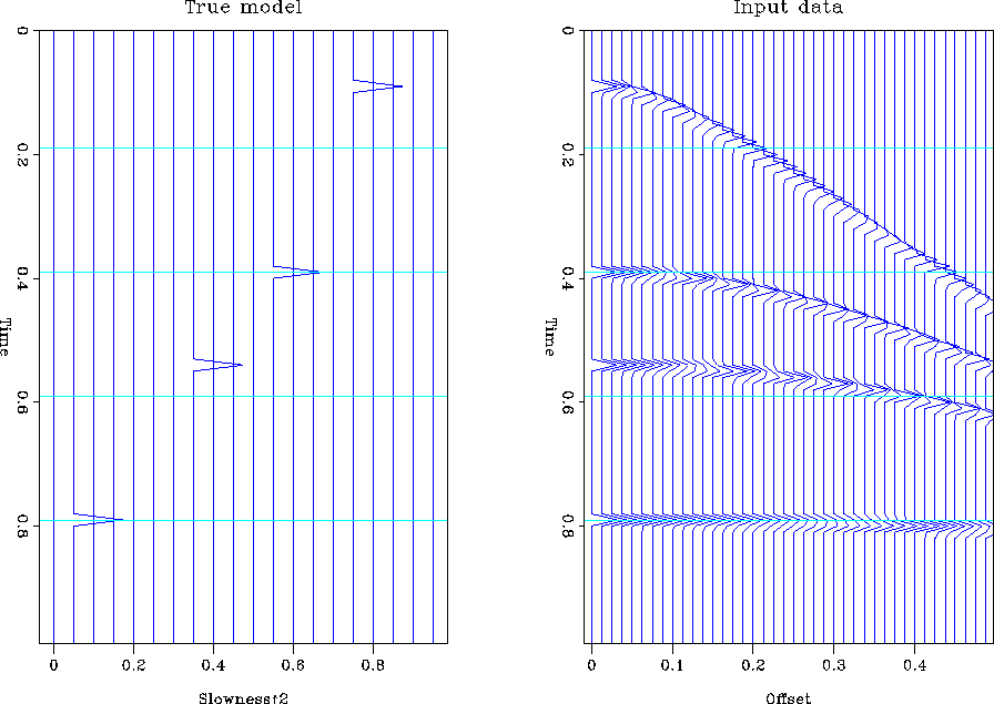
velocity-stack space. Figure synth1 shows a model,
that maps from velocity-stack space to
offset space. If there is spike in velocity-stack space it will create
a hyperbola in the CMP gather. The amplitude of the hyperbola is given
by the height of the spike, the zero-offset time and the moveout of
the hyperbola are governed by the position of the spike in the
velocity-stack space. Figure synth1 shows a model, ![]() , with four
spikes in the velocity-stack space and the corresponding data,
, with four
spikes in the velocity-stack space and the corresponding data, ![]() , in
offset space that is created by the action of the forward operator
, in
offset space that is created by the action of the forward operator
![]() .
.
![]()
 |
For the inverse operator we seek a solution to the problem of finding
the model in velocity-stack space, ![]() , given the data,
, given the data, ![]() . This is usually posed as a least-squares minimization problem
that minimizes the energy of the misfit between the modeled and
measured data:
. This is usually posed as a least-squares minimization problem
that minimizes the energy of the misfit between the modeled and
measured data:
![]()
![]()
![]()
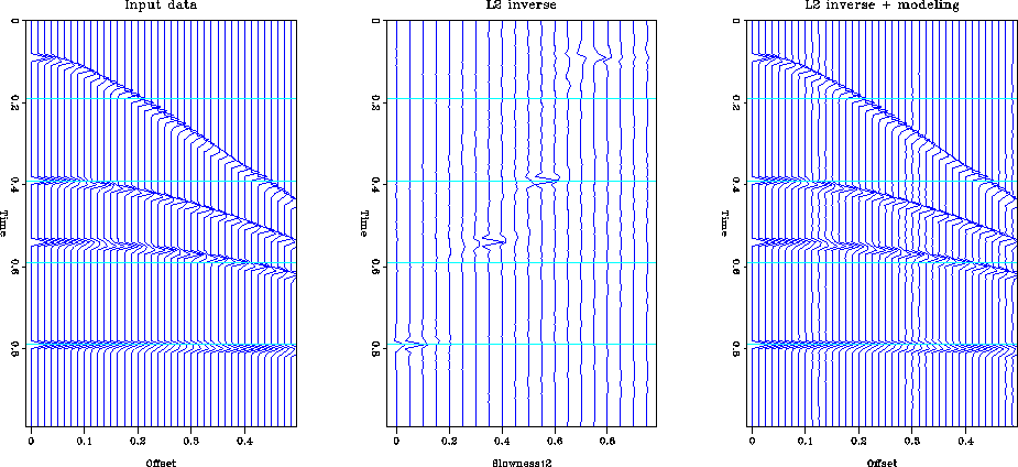
Figure l2synth shows the result of using a conjugate gradient
solver to minimize the L2 norm of the data misfit. The left frame
displays the input data, the center frame shows the inverted data in
the velocity-stack space and the right frame displays the predicted
data from the model. The model predicts the input data very well.
However the inverted model is not the same as the original model data
in Figure synth1. The difference between the two models is in
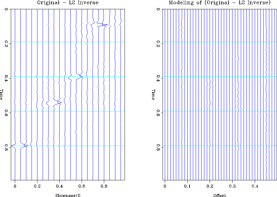
the null space of the operator ![]() . This is easily demonstrated
by taking the difference of the two models and applying the modeling
operator. The result is shown in Figure synth-null. The
original model is not the one chosen by the inversion because it
contains components in the null space.
. This is easily demonstrated
by taking the difference of the two models and applying the modeling
operator. The result is shown in Figure synth-null. The
original model is not the one chosen by the inversion because it
contains components in the null space.
 |
 |
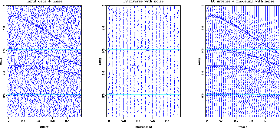
The L2 inversion is the optimal choice in the presence of Gaussian noise. In this case, the L2 inversion gives the maximum likelihood solution to the inversion problem. Figure l2synthn shows the results of L2 inversion when the data is contaminated by Gaussian noise with zero mean and variance of 1/10 of the true model amplitude. The inversion does a satisfactory job of recovering the true model.
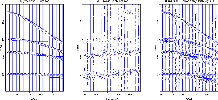
If the noise is not Gaussian then the L2 inversion may not be a good choice. Figure l2synths illustrates the behavior of L2 inversion in the presence of impulsive noise. Four spikes with an amplitude ten times that of the hyperbolas have been added to the input data. The inversion spreads the effect of the spike across the model space. This is especially true of the spikes at the far offset. When the data is remodeled the spikes are not perfectly recreated, they have been smeared into the adjacent traces.
 |
 |
WEIGHTING THE RESIDUAL
The simple L2 norm of the residual is not the only function that we can choose to minimize. We can also choose to minimize a weighted residual
![]()
![]()
The Lp norm
A particular choice for ![]() is one that results in minimizing
the Lp norm of the residual.
Choose the ithdiagonal element of
is one that results in minimizing
the Lp norm of the residual.
Choose the ithdiagonal element of ![]() to be a function of
the ith component of the data vector.
to be a function of
the ith component of the data vector.
![]()
![]()
![]()
![]()
![]()
Since the final residual is not known during the solution of the problem, the minimization is solved using a sequence of weighted least-squares problems. This method is called ``Iteratively reweighted least-squares''. The method has been used before at SEP for deconvolution () but not for velocity-stack inversion. The cost is a little higher than a regular least-squares solver but not excessive.
In practice the reweighting operator is modified slightly to avoid
dividing by zero. A damping parameter ![]() is chosen and the
weighting operator is modified to be:
is chosen and the
weighting operator is modified to be:
![]()
![]()
![]()
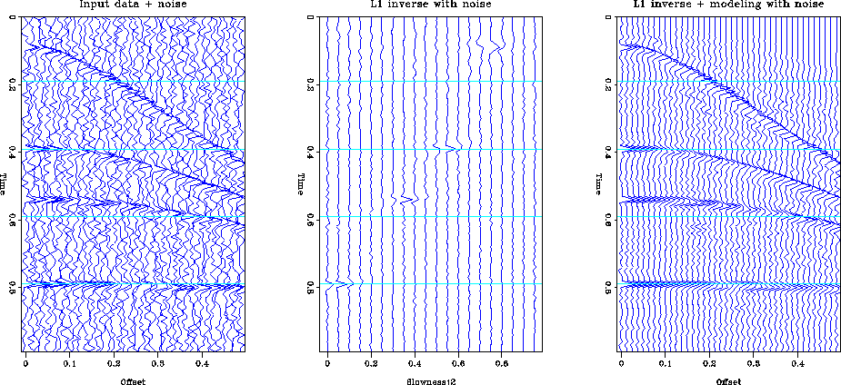
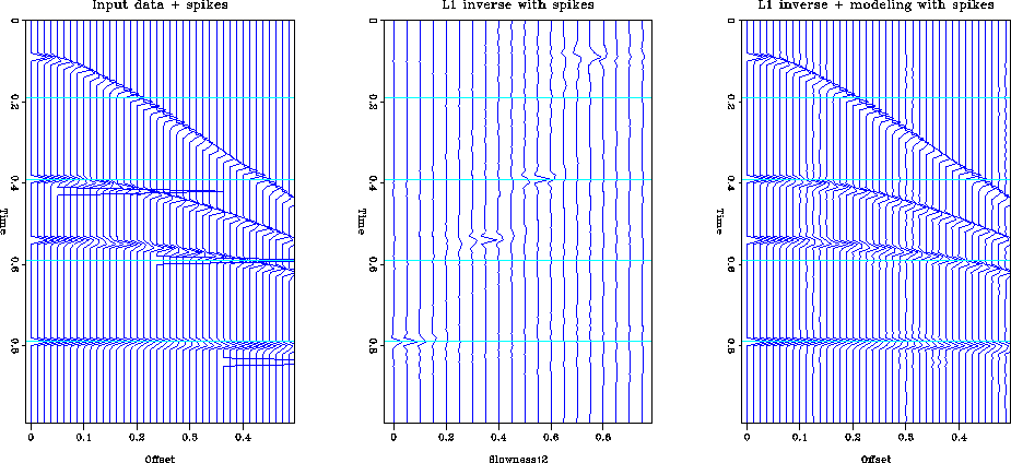
Figure l1synthn shows the result of minimizing a L1.1 data
misfit when the data is contaminated by Gaussian noise, and
Figure l1synths shows the result when the noise is impulsive.
The reconstruction of the data with Gaussian noise is slightly inferior
to the L2 norm. The noise has been concentrated into a few
significant events rather than remaining random. The second example
is the type of problem that L1 methods are best at handling. The algorithm
has completely ignored the spikes in the input data and the
reconstructed data is completely noise free.
However, even though we are estimating a model that minimizes the
L1 norm of the data misfit, we will still be finding the minimum
energy model that satisfies this misfit criterion. The operator
has the same null space as the original operator ![]() so no
energy is added to the null space of the operator. The inverted data
still does not have the spikiness present in the original model.
so no
energy is added to the null space of the operator. The inverted data
still does not have the spikiness present in the original model.
![]()
![]()
 |
 |
WEIGHTING THE MODEL
One way to address the loss of spikiness in the model is to apply a model space weight. Now we solve the problem
![]()
![]()
Minimizing the Lp norm of the model
In the same vein as the previous section we can choose the diagonal
elements of ![]() to be
to be
![]()
![]()
![]()
![]()
![]()
![]()
By combining model space weights and data space weights we can minimize the Lp norm of both the data misfit and the model space. We solve the following problem:
![]()
![]()
This method is implemented using an iteratively reweighted least-squares algorithm that is similar to the previous scheme.
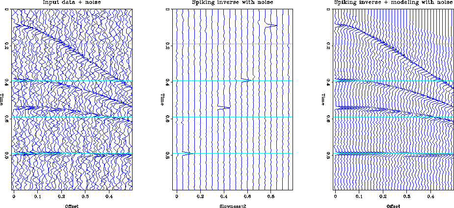
We now have a scheme that minimizes the Lp norm in both the data misfit and the model space.
![]()
![]()
 |
 |
REAL DATA EXAMPLE
The following figures show the effects of using the various inversion methods on one CDP gather from the dataset that was provided for the Mobil AVO workshop. The aim of the inversion is to create an image in the velocity-stack space in which the primary energy and the multiple energy is well separated. In addition the modeled data must be a good match to the primary-only part of the original data. Since this dataset is intended to be used for AVO analysis, it is important that the amplitudes of the events are correctly modeled.
Figure real-l2 displays four stages in the processing of a CMP gather from the Mobil dataset. The first frame is the raw CMP gather, the second frame is its L2 velocity-stack inverse, the third frame is the data remodeled from the inverse, and the final frames is the difference between the input CMP and the remodeled data. The raw data is heavily contaminated by multiples and there are high amplitude bursts at the far offsets. The noise bursts produce long curved artifacts in the velocity-stack space. They are the dominant feature in the inversion and it is difficult to identify the primary velocity trend. However, despite the unpleasant appearance in the velocity-stack space the reconstructed data is a good match to the input and the residual is small over the whole domain. This is the characteristic behavior of L2 inversion, it attempts to minimize the global energy in the residual.
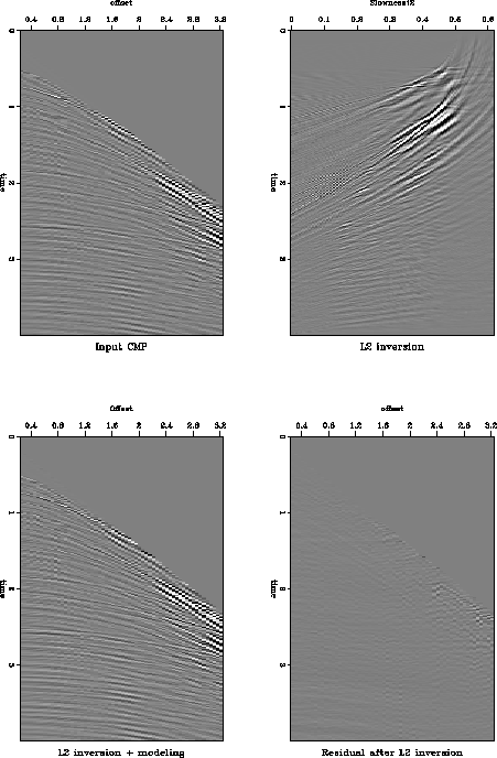 |
Figure real-l1 shows the same four stages of processing when the L1.1 norm of the data misfit is minimized. The model in velocity stack space is still contaminated by the noise streaks but not quite as badly as the L2 inversion. The remodeled data is still a good match to most of the input data but the algorithm has treated the high energy bursts at the far offsets as noise and it has rejected them. The residual energy is higher than in the L2 case, but it is all concentrated in the far offset noise bursts.
 |
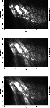
Figure real-spk displays the effect of spiking inversion in the model space. The inversion minimized the L1.1 norm of the data misfit and the L1.1 norm of the model. The events in velocity-stack space are much more compact and the noise streaks do not cross the trend of the primary energy. This is a very desirable result, if we intend to mute the data in velocity-stack space. It is much easier to separate the primary trend ( to the left of the figure) from the multiples and the effects of the noise bursts.
 |
The differing concentration of the energy can be seen more clearly be examining the envelope of the data in velocity-stack space. Figure realenv compares the envelope of the data for the three inversions. The result of spiking inversion shows a much better separation of primary and multiple data.
 |
![[*]](http://sepwww.stanford.edu/latex2html/movie.gif)
DISCUSSION
The choice of a suitable norm for data misfit is dependent on your expectations of the the noise character. If the noise is known to be Gaussian and uncorrelated, it is best to minimize the L2 norm of the data misfit. If the noise is expected to be impulsive, it is better to minimize a lower order norm. I have shown that for noise that is pure spikes the L1.1 norm was very successful: it completely eliminated the spikes.
The same considerations apply to the norm of the model. If the model is expected to be smooth, then a L2 norm may be appropriate. If the model that you desire is spiky, a L1.1 norm may be more to your taste.
An advertisement for C++
All of the iterative solver routines developed for this work were written within the ``CLOP'' framework (). This means that the solvers are now available for use with any operator written within that framework. The same routine can be used with velocity-stack operators, convolutional operators, migration operators etc. This is in sharp contrast to many problems coded in Fortran for which a new solver often needs to be implemented for each new operator.
[SEP,SEGCON,GEOTLE,SEGBKS,MISC]
![[*]](http://sepwww.stanford.edu/latex2html/prev_gr.gif)