#1to.2ex~

#1#1

Statics prediction from cross-correlations in orthogonal directions

Ray Abma

Author has no known email address

ABSTRACT

Traditional reflection statics programs use model traces built from stacks of nearby traces. Using cross-correlations between nearby prestack traces avoids the problems associated with the model building process. Cross-correlations between trace pairs positioned in orthogonal directions with respect to structure, residual NMO, and the shot and receiver terms allow the full statics problem to be separated into three sets of problems. Cross-correlations are performed in gathers that are independent of, or orthogonal to, one of three parts of the full problem. These simpler problems may be solved individually with greater ease and perhaps with more accuracy than traditional approaches. Since only one term is being predicted within each subset of the problem, this may be considered a signal-processing problem rather than a matrix-inversion problem. The cross-correlations of neighboring traces may be supplemented with the creation of cross-correlations between traces that are widely separated. These extra cross-correlations may stabilize the problem. Preliminary results on synthetic data appear promising.

Poorly consolidated, low-velocity near-surface layers with properties that vary widely from one surface location to another often distort seismic wave fields that pass through them, corrupting the image of the subsurface below. The velocity of this weathering layer tends to be much lower than that of the layers below, making the ray paths through this layer approximately vertical. Since the ray paths are almost vertical, the corrections for the travel path through the weathering layer may be approximated by a single time shift at each surface location. This time shift is referred to as a static correction, as opposed to dynamic corrections such as NMO.

Traditional reflection static techniques rely on time shifts taken from traces correlated against a model trace. This model trace is generally built by stacking traces near the point of interest. The calculated time shifts are then used in a matrix inversion to solve for the static shifts caused by the weathering layer (, ). The quality of the model, which is built without static information and generally with a poor knowledge of the velocity field, determines the quality of the results.

One alternative to the traditional approaches is simulated annealing, which is used to calculate statics by stacking with a series of random statics without a previously defined model(). This technique tends to be expensive and appears to be most commonly used without residual NMO corrections. The solutions may also suffer from low-frequency instabilities which must be filtered out of the final result.

The refraction statics techniques take advantage of the refracted arrivals from the near-surface layers to create a model of the near surface. This model is then used to derive reflection statics. Refraction statics assume good refracted arrivals from fairly regular near-surface layers without velocity inversions. Bevc pointed out that transmitted arrivals which are mistaken for refracted arrivals cause substantial errors in the calculated statics. Also, once the near surface becomes complicated enough to make first arrivals incoherent, standard refraction static methods will fail().

Musser et al. suggested a technique that utilized cross-correlations between neighboring traces and discussed extending the cross-correlations beyond adjacent traces. This method has similarities to the technique presented in this paper, but the solution to the problem was still based on a solution to a single large matrix problem.

In the technique I suggest here, prestack traces are correlated against nearby prestack traces in directions that minimize the effects of one of the solution's terms. For example, traces cross-correlated within a common-midpoint gather are assumed to be unaffected by the structure term. Traces cross-correlated within a common-offset gather are almost independent of the residual NMO term. Within a common-receiver gather, trace-to-trace correlations minimize the receiver statics.

Once a particular term is minimized, another term may be extracted using processes that are closer to signal processing techniques than to matrix inversion. Here, I divide the static problem into three sets of problems. The first two problems sets determine the residual NMO and the structure terms, which may be separated by cross-correlating traces within the common midpoint gathers and within the common-offset gathers. The third problem set determines the shot and receiver terms, which are combined into a single weathering term. By cross-correlating within the shot and receiver gathers, the two terms may be derived without interfering with each other. This technique may be viewed as an extension of what a human does when he or she picks statics by hand from common shot and receiver gathers.

If this process is viewed as a matrix inversion problem, the solution to the smaller parts of the problem approximate the total solution. Iterating the solutions to these smaller problems allows the cross terms to be accounted for in the full matrix inversion problem. Cross-correlating between prestack traces may allow a less singular matrix to be inverted, since the matrix may be filled out by creating more cross-correlations along the orthogonal directions using non-adjacent trace pairs.

In this paper, I outline a possible approach for solving the statics problem using these techniques. The connections between the terms to be removed and the various gathers in which cross-correlations are done within are shown. In particular, the connection between the residual NMO and the structure has a more complicated relationship than the relationships between the other terms. A technique for breaking the matrix-inverse problem into three smaller problems is given. The form of the matrix generated by increasing the number of cross-correlations is shown to improve the properties of the static predictions in the presence of noise. The preliminary results on synthetic data appear promising, since the residual NMO, structure, and weathering terms were well predicted in that case.

ORTHOGONAL CROSS-CORRELATIONS

Cross-correlating between unstacked traces

Rather than using the traditional approach of deriving time-shifts from the cross-correlations between a model trace and unstacked traces, the technique suggested here uses the relative static time shifts from picks of cross-correlations between various unstacked traces (). Deriving relative static shifts is a less direct approach for getting the desired result, since the final static solution results from an integration of the relative statics, but this technique does not suffer from the errors introduced by building a model trace.

When the static shifts are large, the process of building the model trace may need to go through several iterations before an acceptably good model is generated. The cross-correlations between prestack traces will not change with the change of calculated static values, so the costly processes of stacking and correlating need not be repeated.

The simplest model is an ordinary stack of the data using whatever velocity field is available. If relative static shifts are large, the traces in a simple model made from the stack of nearby traces may become incoherent. Although shifting the traces for maximum coherence in stacking will help with small static shifts, cycle skipping occurs when the relative shifts become larger than the dominant wavelength. Residual NMO terms can produce errors in the structure term of the model if the distance to the nearest offset is significant. Although the picks from relative cross-correlations are likely to suffer more from noise in the prestack traces, increasing the number of cross-correlations within each gather may compensate for this disadvantage.

An analogy to picking hand statics

Another way of looking at cross-correlating non-adjacent traces is to compare it to the method a human would use to derive statics. Rather than comparing pairs of traces within a shot or receiver gather, a human will look at an entire gather, attempting to find the shift from a single surface location by comparing a trace to a number of traces in the neighborhood. A single bad trace will not significantly hinder his or her work, since any individual trace is compared to many nearby traces. While a human will generally confirm a static shift by comparing several gathers, the problem becomes a three- or four-dimensional puzzle, with a tremendous amount of information to be considered. The advantage of the computerized version of this approach is that the computer can consider multiple gathers simultaneously to predict a single static value, while a human has the time and patience to consider the shifts within only a few gathers. For the residual NMO term and the structure term, one more dimension is available by considering a single shift term in many gathers. For the weathering term, two extra dimensions are available, one along the shot axis and one along the receiver axis. When the acquisition becomes three-dimensional, each problem gains one or two more dimensions of complexity, generally overwhelming a human's capabilities.

Term separation in orthogonal directions

While others have used trace-to-trace cross-correlations () and (), I separate the various terms of the problem using relative shifts from traces cross-correlated in directions that allow one term of the unknowns to be ignored. For example, the traces within a common-shot gather have relative shifts that are not affected by the shot time shifts; the receiver static time shifts have no effect. A similar situation is true for the relative time shifts in a common-receiver gather.

Only one term is removed by the cross-correlations in a particular direction. Ideally, all but one term would be removed from the measurements. Since this is not possible, the problem is broken into three parts: one part considering just the residual NMO, one part considering just the structure term, and one part considering just the weathering term which produces the shot and receiver statics. Since the residual NMO and the structure terms are more closely related to each other than to the weathering term, they are more likely to interfere with each other. To avoid this interference, the structure term is eliminated for the residual NMO calculations, and the residual NMO term is eliminated for the structure term calculations. The weathering term appears as noise, which is assumed to be uncorrelated with the other terms.

The separation of the residual NMO and structure terms from the weathering term is reasonable, since the shot and receiver statics tend to contain high spatial frequencies, and the residual NMO and the structure terms tend to contain lower spatial frequencies. Once the low frequency terms are eliminated, the shot and receiver terms can be separated by cross-correlations along the receiver and shot gathers to make the predictions of the weathering statics simpler. The three parts of the problem are assumed to be only weakly dependent. Whatever relation exists between these parts is resolved by iteration.

In this technique, some information about a term to be calculated is ignored to simplify the problem. Only the information derived from a gather most suited to calculating the term of interest is used. While some information is thrown away, many cross-correlations may be generated within a gather to supplement the solution.

Gather types and cross-correlation directions

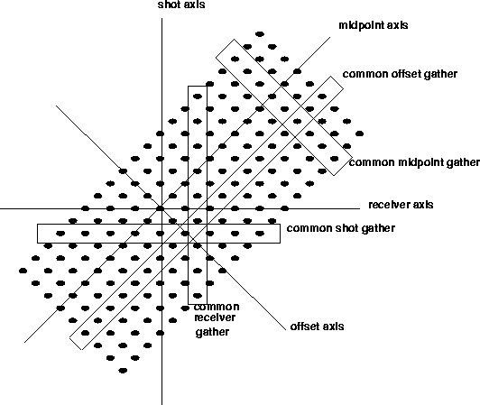
A two-dimensional seismic line actually contains several more dimensions. While the final result shows only the dimensions of midpoint location and depth, offset provides an additional dimension to the intermediate problem. As seen in Figure gathers, the midpoint and offset axes may be transformed into shot and receiver axes. Each of these coordinate systems have advantages in applying certain processes. For the statics problem, I take advantage of these coordinate systems to simplify the problem.

As a review, the common-midpoint gathers are collections of traces with the same midpoint between shot and detector. A common-offset gather contains all the traces with an equal shot to detector distance. A common-shot gather contains all the traces from one shot. The common-receiver gather contains all the traces that were recorded at one position at the surface, not necessarily those from a single detector.

 

gathers
Figure 1 The various coordinate systems used to describe a 2-D seismic line. After FGDP.

PROCESSING STEPS

Calculating the residual NMO term

The residual NMO may produce larger time shifts than the other terms, since the velocity field tends not to be well known, and small velocity errors can create large shifts on the far offsets. Since a velocity error will produce a trace-to-trace shift within a common-midpoint gather that is approximately linear, a simple fit to a linear function may be used to derive the residual NMO. The derived residual NMO is forced to be a smooth function with respect to the CMPs.

I have two approaches for calculating the residual NMO. The first approach is to simply sum weighted values of the trace-to-trace shifts within a common-midpoint to get an average value for the residual NMO in each common-midpoint. The results are then smoothed along the common-midpoint axis to insure that the result contains only long spatial wavelengths. The contributions of the shot and receiver statics are assumed to average out in this part of the problem. If they do not, more iterations of the steps may be needed.

The approach used in the examples shown later in this paper uses a matrix inversion technique that allows low fold gathers and near traces to be weighted down. It also allows weighting the problem to insure that the results are smooth. This approach provided more flexibility for this preliminary version of the program, although the results of the two approaches were generally similar.

Calculating the structure term

The structure term is calculated from common-offset gathers, which, as pointed out by Muir , should show little effect from the NMO term. Muir points out that the entire statics problem may be solved using only terms derived from common-offset gathers. His approach does not require NMO to be applied before statics are calculated and velocities determined. In this paper, I approach the problem in a more conventional manner, choosing to apply NMO and calculating what is hopefully a small correction.

While the shot and receiver statics are considered orthogonal to each other, the residual NMO and the structure terms are only approximately independent. Within a common-midpoint gather, the trace-to-trace time shifts may be considered independent of the structure. In a common-offset gather, the relative trace shifts are approximately independent of the residual NMO term only if the residual NMO is almost constant. If there is a rapid change in the residual NMO along the CMP axis, this change in the residual NMO will appear in the structure terms. (See the synthetic example in Figures Figa and Figb.) This effect of the residual NMO should be removed from the structure term to correct for the changing residual NMO. While changes in the structure term may affect the velocity, the effect is much smaller and is ignored. The shot and receiver statics are considered noise in this problem.

In the results shown here, the differential residual NMO was first removed and a correction to the common-offset cross-correlation panels was made. Then a simple average of the differential structure terms within each common-midpoint gather was made, and the values were smoothed along the common-midpoint axis. The final structure values calculated result from an integration of the differential structure values.

Calculating the weathering term

Once the corrections for residual NMO and structure are made, surface-consistent static shifts are calculated. The relative static values may be determined by simply averaging the picks or by using a median value if the surface station increments are equal to one station within the common-shot and receiver gathers. Since the receiver gathers are likely to have shot increments greater than one station, and cross-correlations may be generated across non-adjacent traces, I use a matrix inversion technique to calculate the statics, although other techniques, such as an inverse filter calculated to account for the geometry, could be used.

While the shot and receiver terms were considered as noise in the residual NMO and structure term calculations, the remaining residual NMO and structure terms are considered noise in this problem. More iterations may be needed to completely separate the terms.

Iterations of the previous problems

While the residual NMO, structure, and weathering terms may be considered to be relatively independent of each other, there will be some interdependencies between the terms, since the random changes in one term will appear as noise while calculating another. The individual problems of deriving residual NMO, structure, and weathering terms then must be iterated to improve the results as the noise from the other terms is reduced. Even if the relation between the terms is not random, iteration may be used to redistribute the values of the terms.

An advantage of this method over traditional methods is that the relative picks between prestack traces will not change as the solution is improved. In the traditional methods that use model traces against which the prestack traces are correlated against, each improvement of the solution should be accompanied by the rebuilding of the model. In practice, only a few iterations of model building are generally used.

CROSS-CORRELATING NON-ADJACENT TRACES

Noise attenuation

One advantage of the technique I present here is that the solutions to the various terms of the task may be approached as a signal processing problem rather than as a matrix inversion. Signal processing techniques such as median filtering are simply applied to the individual terms of the solution; the process is easier to visualize and understand, and the process is more robust in the presence of noise.

If data were recorded without noise, the static prediction problem would be greatly simplified. Unfortunately, as the near surface becomes more complicated, static shifts grow larger, and more noise is generated by scattering. Since scattering is produced in three dimensions of the near surface and a time shift is produced by only one dimension, the scattering noise increases rapidly as the static shifts grow. While some of the scattering noise will appear as extensions of the wavelet associated with a surface location, some of the scattering will appear as incoherent noise.

In traditional statics predictions, the model traces are built using many nearby traces to reduce the noise in the model trace. The prestack traces correlated against the model trace still suffer from the noise. In the approach suggested here, there is no noise attenuation done before picking the cross-correlations, but it is hoped that using many picks will produce an average pick that is approximately correct. However, this is not necessarily true, and other methods of deriving a typical pick may be needed.

Computing additional cross-correlations between traces that are not adjacent should produce better results in the presence of noise, but there is a limit to the distance that time-shift measurements between prestack traces are useful. One of the assumptions in this technique is that nearby traces are similar. Once the distance between traces becomes so large that important similarities are lost, measuring the time shifts between the traces becomes almost meaningless. An alternative view is that there should be enough separation for the noise on the two traces being cross-correlated to be independent. In practice, uncertainties in identifying the source and the spatial range of the noise force a range of trace separations to be used.

This technique as a matrix problem

The form of the matrix to be inverted when cross-correlating prestack traces is different from the form of the matrix used in the traditional approach (, ) in which each prestack trace cross-correlated against a model trace generates a time-shift value to become one equation in the system or one row of the matrix. By using relative cross-correlations between unstacked traces, many more time-shift measurements can be produced. This generates more equations in the system, or more rows in the matrix, while retaining the same number of unknowns, making the system more robust in the presence of noise as it becomes more over-determined. If this system of equations was described by $\bf y = \st A \bf x$,the least-squares solution is $\bf x = (\st A^{ \dag } \st A)^{-1} \st A^{ \dag } \bf y$.The matrix to be inverted, $(\st A^{ \dag } \st A)$, is the same size in both the traditional case and with the technique suggested here, so the cost of solving for the static shifts will be similar for both techniques if the cost of correlating the prestack traces and building the model traces are not included.

While the solution to the system of equations may be solved by calculating $(\st A^{ \dag } \st A)^{-1}$ or by solving the equivalent problem iteratively, as in Musser et al. , I suggest a solution of smaller parts of the problem by techniques more related to signal processing than matrix inversion. The full solution then involves an iteration of these separate solutions.

For short lines, solving the full least-squares matrix inverse problem exactly is a practical approach. For larger lines, the memory and computational requirements become infeasible, or at least, inconvenient. An alternative to the exact solution is the result of the first few iterations of an iterative approach, such as conjugate-gradient or Gauss-Seidel (). In the technique presented here, the larger problem is solved by iterating exact solutions of three smaller problems, those of residual NMO, structure, and weathering.

If these three problems were independent of, or orthogonal to, each other, only one iteration would be needed. Some dependence exists between the separate problems, however. To solve the three problems simultaneously, the solutions to the separate problems are iterated. Since the individual problems are fairly small and exact, each iteration should not be excessively costly.

The order of the solution of the smaller problems is to first solve for the residual NMO terms, then solve for the structure terms, and finally calculate the shot and receiver terms. While the problem could be solved with other orderings, it can be argued that the residual NMO terms can produce the largest time shifts and should be done first. If the shot and receiver statics have a zero mean, the structure calculations should be insensitive to the them and could be solved next. The shot and receiver statics are calculated after the other two sets of problems. If these assumptions are incorrect, more iterations of the three sets of small problems will be needed, but the problem should still converge to the correct solution.

Creating more measurements by making cross-correlations between traces that are not adjacent may be considered as a modification of the $(\st A^{ \dag } \st A)$ least-squares matrix for the inverse problem. As more cross-correlations are used, the $(\st A^{ \dag } \st A)$ matrix is filled out, perhaps making the problem less singular, as well as stabilizing the process against noise and improving the long-wavelength static solutions.

The computational time needed to get a solution to the full matrix equation is proportional to n³, where n is the number of unknowns. For typical two-dimensional seismic lines, n will vary from a hundred to many thousands. Breaking the problem into smaller parts will significantly reduce the cost if the connection between the parts of the problem is weak. In this case, only a few iterations of the smaller parts of the problem are needed. If the connections are strong, more iterations will be needed.

EXAMPLES

A synthetic example

A simple synthetic was constructed for testing the various programs used to derive static shifts. A single surface static with a smooth residual NMO and structure term was used in this model. These terms are shown in Figures struc and statics. These shifts were applied to a simple synthetic dataset containing forty shots, which were then cross-correlated and picked. The picks were then used to predict the static, the residual NMO, and the structure terms.

The picks derived within the various gathers are shown in Figures Figa to Figd. Figure Figa shows the picks done within CMP gathers. These picks are not affected by the structure terms, so it does not appear in this figure. Figure Figb shows the picks done within common-offset gathers. The structure term is now apparent. Even though it should be weak, the residual NMO term is obvious in this figure because the residual NMO term changes rapidly along the CMP axis in this example. Figure Figc shows the picks from the cross-correlations done within shot gathers, so the vertical line corresponding to the shot static is not seen. Likewise, Figure Figd shows the picks from the cross-correlations done within receiver gathers, so the diagonal line from the receiver static is not seen.

 

Figa Figure 2 Time shifts seen in cross-correlations within CMP gathers. White indicates a positive time shift; black indicates a negative shift. These cross-correlations are not affected by structure terms, so the structure term is not seen here. Compare to Figures 3 to 5.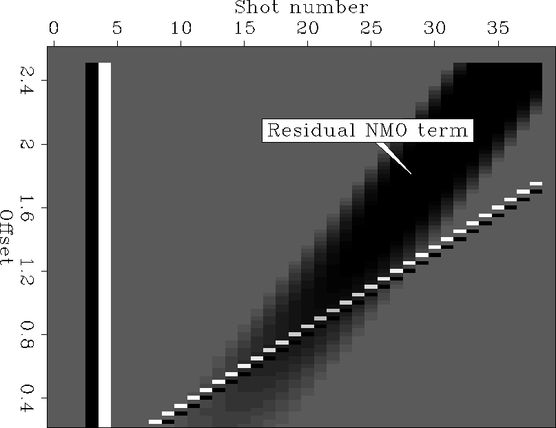

 

Figb Figure 3 Time shifts seen in cross-correlations within common-offset gathers. These cross-correlations are weakly affected by the residual NMO terms, as can be seen by the existence of the residual NMO effect.

 

Figc Figure 4 Time shifts seen in cross-correlations within common-shot gathers. These cross-correlations are not affected by the shot statics, so the vertical line caused by the shot static is not seen here. Compare to Figure 5.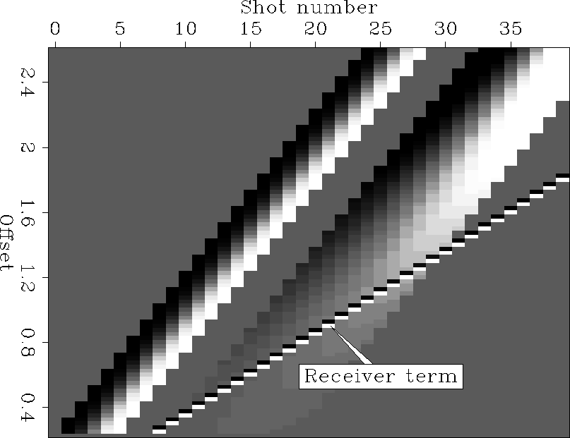

 

Figd Figure 5 Time shifts seen in cross-correlations within common-receiver gathers. These cross-correlations are not affected by the receiver statics, so the diagonal line caused by the receiver static is not seen here. Compare to Figure 4.

Figure resa shows the picks from the common-offset gathers after the calculated terms are removed. Notice that only weak events remain. This lack of strong features indicates that the process has been successful.

 

resa Figure 6 Time shifts seen in cross-correlations within common-offset gathers after correction for the calculated static problem terms.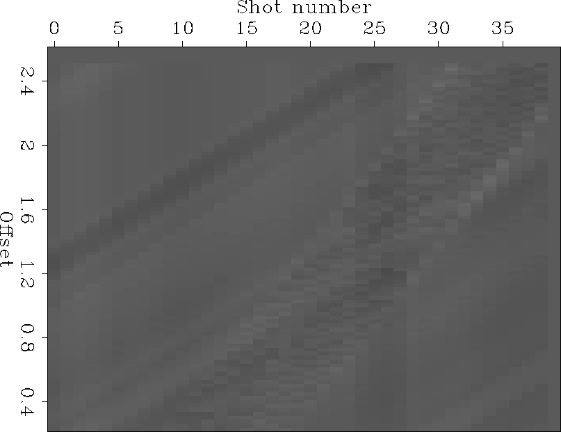

The calculated residual NMO and the structure terms seen in Figure calstruc are close to the original residual NMO and the structure terms seen in Figure struc. The small remaining differences may be due to the smoothness constraints used in the calculations. Since there was no visible difference between the original statics in Figure statics and the calculated statics, the calculated statics are not shown. Only one iteration was used to produce these results.

 

struc Figure 7 The residual NMO and the structure terms used to create the simple synthetic. The small, narrow peak on the left shows the structure term, and the larger, wider peak on the right shows the residual NMO term.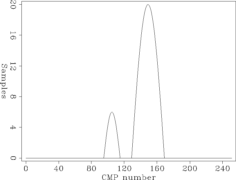

 

calstruc Figure 8 The residual NMO and the structure terms calculated by the statics program. The small, narrow peak on the left shows the structure term, and the larger, wider peak on the right shows the residual NMO term.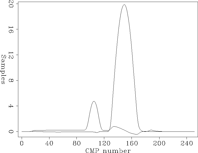

 

statics Figure 9 The surface static term used to create the simple synthetic. The calculated result showed no visible difference.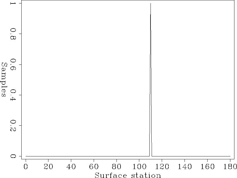

While the statics on a simple synthetic could be calculated successfully, complicated synthetics showed some problem separating residual NMO and structure from the weathering that iteration did not resolve. Part of this failure may be due to the inherent singularity of the matrix being inverted, but some of it may be due to the lack of constraints placed on the RNMO and structure terms.

A real example

A real dataset provided by Conoco that was used by Rothman in his simulated annealing work and described in Bally had the data cross-correlated in the same manner as the synthetic example previously described. The results are shown in Figures Wyo1 to Wyo4. These figures correspond to Figures Figa to Figc of the synthetic example. Although suggestive patterns can be seen in the Conoco data, picking errors produce enough background noise to make identification of events difficult. Even more troublesome is the inconsistency of the events seen on one of the figures when compared to the others.

 

Wyo1 Figure 10 Time shifts seen in cross-correlations within CMP gathers in the Conoco dataset. Compare to Figure 2.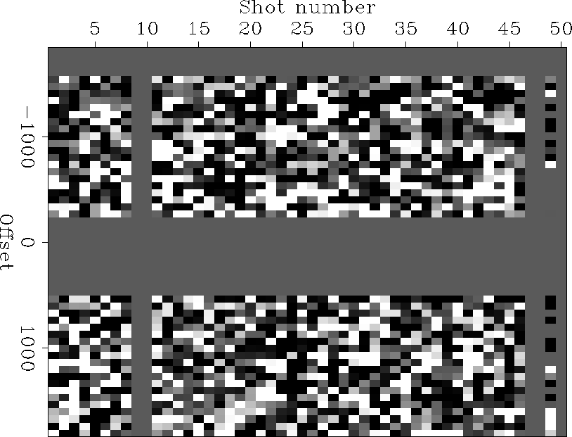

 

Wyo2 Figure 11 Time shifts seen in cross-correlations within common-offset gathers in the Conoco dataset. Compare to Figure 3.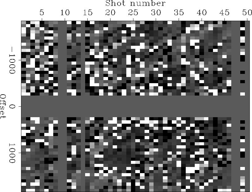

 

Wyo3 Figure 12 Time shifts seen in cross-correlations within the common-shot gathers in the Conoco dataset. Compare to Figure 4.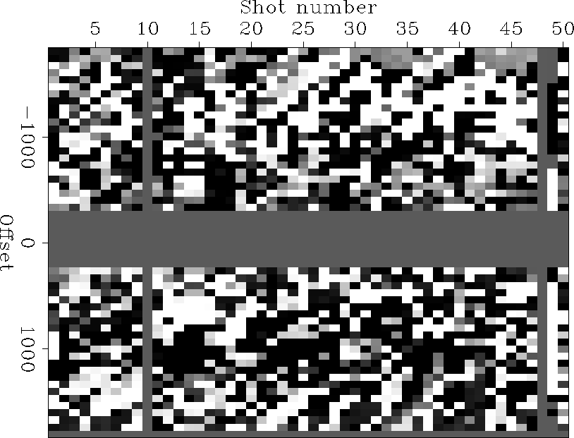

 

Wyo4 Figure 13 Time shifts seen in cross-correlations within common-receiver gathers in the Conoco dataset. Compare to Figure 5.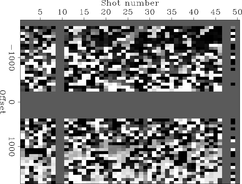

I tried calculating and applying only the weathering statics on this dataset, ignoring the residual NMO and structure terms. The results seen on the corrected gathers were only slightly changed, and no obvious improvements were seen on the stacked results, neither of which is shown here. The simple preliminary version of the program used to calculate the statics from the picks is likely to be the cause of this failure, especially since the picks appear noisy. At the time this paper was written, the individual statics problems were being solved with simple summing or matrix inversions, without weighting for the quality of the picks and without removing outlying picks. It is expected that more work will overcome these difficulties.

EXTENSIONS

As was previously mentioned, the techniques suggested here allows the inversion to be approached as a signal processing problem. As such, I would like to add median filters to the predictions of the various terms. For the residual NMO and structure terms, calculating the medians is straightforward, since the low spatial frequency allows predictions by simple sums. The weathering terms provide more of a challenge, since they contain higher spatial frequencies, but it still can be approached in a similar manner.

The extension of this technique to three-dimensional surveys is straightforward. While more cross-correlations will generally be used in a three-dimensional survey, the information from the cross-correlations in the extra dimension should allow more robust results in the presence of noise.

Removing noise from the prestack traces would be the ideal solution, but the time shifts between traces make this difficult. Processing the cross-correlations themselves rather than just using the picks from the cross-correlations may allow more reliable results. The problem here is how best to combine the information from the many cross-correlations (). Muir suggested that the envelopes of the cross-correlations be used to derive more reliable statics, since they could be combined in a straightforward manner.

One possible disadvantage of this technique is that a bad data zone may introduce spurious time shifts between the reflections on either side of the zone. While these shifts may be removed by adding assumptions about the structure of the solution, it complicates the problem.

CONCLUSIONS

I have developed a technique that shows promise in providing better solutions to static problems due to weathering irregularities. This process makes use of cross-correlations between unstacked traces in directions that allow various terms of the solution to be ignored, simplifying the inverse problem by dividing the problem into smaller problems with more straightforward solutions. I suggest increasing the number of cross-correlations within a gather to include nonadjacent traces may stabilize the problem in the presence of noise. More cross-correlations may also improve the long-period statics by making the matrix being inverted less singular.

Using median filters and removing outliers from the calculations may improve the results in the real dataset I considered. Finally, without experience with a large number of real datasets, the utility of this method is difficult to judge. This technique should be tested on a variety of real problems to gain a better understanding of its limits and strengths.

ACKNOWLEDGMENTS

I thank Francis Muir for his suggestions on approaching statics determination problems. I would also like to thank Thorbjørn Rekdal and Luis Canales for many helpful discussions of issues related to near-surface problems. Thorbjørn also had many useful suggestions for improving this paper. Finally, Conoco deserves thanks for making the Wyoming dataset available.

[mybib]