Modeling 3-D anisotropic fractal media

Nizar Chemingui

Author has no known email address

ABSTRACT

This paper presents stochastic descriptions of anisotropic fractal media. Second order statistics are used to represent the continuous random field as a stationary zero-mean process completely specified by its two-point covariance function. In analogy to the two-dimensional Goff and Jordan model for seafloor morphology, I present the von Karman functions as a generalization to media with exponential correlation functions. I also compute a two-state model by mapping the random field from continuous realizations to a binary field. The method can find application in modeling impedances from fractal media and in fluid flow problems.

Our understanding of the physical phenomena occurring in the earth always involves the study of the medium itself. Unfortunately, the earth offers an unusually complicated medium in which heterogeneities are observed at every scale. Sometimes the problem is too difficult to deal with deterministically but it turns out to be quite simply treated by statistical methods. Solutions to the one-dimensional problem have targeted the study of reflectivity series obtained from well logs. Seismic impedance can be modeled as a special type of Markov chain, one which is constrained to have a purely exponential correlation function (). The two-dimensional problem has gained a lot of attention in the recent years from studies of seismic scattering in heterogeneous media, e.g., (, , , , ). Three dimensional simulations can be used in fluid flow experiments ().

This paper presents a method for simulating three-dimensional anisotropic random fields using second order-statistics. The method was introduced by Goff and Jordan (1988) to model a two-dimensional seafloor morphology. I have considered the cases of random media characterized by Gaussian, exponential and von Karman correlation functions. I use the von Karman functions as a generalizations to the exponential correlation functions in modeling random sequences. This type of correlation function was first introduced by von Karman (1948) for characterizing the random velocity field of a turbulent medium. It has since been frequently used in the statistical literature, studies of turbulence problems, e.g.(), and studies of random media such as wave scattering, e.g.(). The von Karman functions were identified specifically as belonging to the class of continuous correlation functions (). Holliger et al. (1993) used von Karman covariance functions to model binary fields and defined ``binarization'' as a mapping of all values in a continuous field to just two values of the new field. I have employed their technique to model two state models (i.e, rock/pore or sandstone/shale) from continuous realizations and test the increase in medium roughness through the ``binarization'' process.

RANDOM FIELDS

A stochastic model is constructed for the properties of the random medium. We first construct a distribution function P(x) for the properties of the medium h(x). From such a probability function, we can recover the statistical properties of the distribution (i.e., mean, variance , etc.) through its N-point statistical moments ().

$$\begin{eqnarray} C_N(x_1,x_2,...,x_N)& =& <h(x_1)...h(x_N)\gt \nonumber \\ & =&... ...ty}...\int_{-\infty}^{+\infty}h_1...h_NP( h_1, ...,h_N)dh_1...dh_N\end{eqnarray}$$ (1)

where h_N=h(x_N). The key assumption of spatial homogeneity (stationarity) means that the N-point moments are taken to depend only on the vector joining these points and not on their absolute positions. These moments describe the magnitude and smoothness of the fluctuations of h(x).

Second-order Statistics

I restricted this research to the study of second-order statistics of random fields. This means the study of random media characterized by Gaussian distributions, where a Gaussian process is completely specified by its first- and second-order moments. Furthermore if I define the field h(x) to be a zero mean process:  

$$<h(x)\gt=\int_{-\infty}^{+\infty}h(x)P(h(x))dh=0 \\ end{displaymath}$$ (2)

then h(x) is fully described by its two-point moment that is its autocovariance function which we write as a function of the correlation function:  

$$C_{hh}(r)=E[h(x)h(x+r)]=H^2\rho_{hh}(r) \\ end{displaymath}$$ (3)

where P(h(x)) is the probability density function of h(x), r is the lag vector, E is the expected value, H² is the variance (i.e. C_hh(0)) and $\rho_{hh}$ is the three-dimensional correlation function. Equation (3) shows that the random medium can be adequately specified by its autocorrelation function. More generally, an anisotropic random field can be described by a monotonically decaying autocorrelation function whose rate of decay depends on direction. The roughness of the medium is function of the decay rate of the correlation. The Fourier transform of the autocorrelation is the power spectrum of the field (). Three types of correlation functions were commonly used in the field of seismic modeling: the Gaussian, exponential and von Karman functions. These special functions are described by analytic expressions of their autocorrelations and Fourier transforms.

Two-dimensional cases have been studied for some time (, , , , ). Within the last several years, computer capacity and speed have grown rapidly. It is now feasible to extend our models and simulations to the three-dimensional case.

von Karman correlation functions

The three-dimensional anisotropic von Karman function is given by ():  

$$C(r)=\frac{4\pi{\nu}H^2r^{\nu}K_{\nu}(r)}{K_{\nu}(0)} \\ end{displaymath}$$ (4)

and its three-dimensional Fourier transform is:  

$$P(k)=\frac{4\pi{\nu}H^2}{K_{\nu}(0)}\frac{a_x^2+a_y^2+a_z^2}{{(1+k^2)}^{\nu+\frac {3} {2}}} \\ end{displaymath}$$ (5)

where $r=\sqrt{\frac{x^2}{a_x^2}+\frac{y^2}{a_y^2}+\frac{z^2}{a_z^2}}$, $k=\sqrt{k_x^2a_x^2+k_y^2a_y^2+k_z^2a_z^2}$; a_x, a_y and a_z are the characteristic scales of the medium along the 3-dimensions and k_x, k_y and k_z are the wavenumber components. $K_\nu$ is the modified Bessel function of order $\nu$, where $0.0<\nu<1.0$ is the Hurst number (, ). The fractal dimension of a stochastic field characterized by a von Karman autocorrelation is given by:  

$$D=E+1-\nu \\ end{displaymath}$$ (6)

where E is the Euclidean dimension i.e., E=3 for the three-dimensional problem. The special case of $\nu=0.5$ yields to the exponential covariance function that corresponds to a Markov process ().  

$$C(r)=H^2e^{-r} \\ end{displaymath}$$ (7)

whose three-dimensional Fourier transform is given by:  

$$P(k)=H^2\frac{a_x^2+a_y^2+a_z^2}{{(1+k^2)}^{2}} \\ end{displaymath}$$ (8)

karmanheight=3.5in,width=5.inComparison of 1-dimensional isotropic von Karman autocorrelation functions for varying hurst number, $\nu$.Decreasing the Hurst number, $\nu$, increases the roughness of the medium. The limiting cases of unity and zero correspond to a smooth Euclidean random field and a space-filling field respectively.

Figure karman shows the one-dimensional isotropic von Karman correlation function plotted for different values of $\nu$. The functions have exponential behavior but different decay rates. The higher the slope, the rougher the medium (i.e., the lower is $\nu$). The exponential behavior is explained by the modified Bessel functions $K_\nu(x)$ which in the region $x \gg \nu$ behave as  

$$K_\nu(x) \approx \frac {1} {\sqrt{2\pi x}} \exp{(x)} \\ end{displaymath}$$ (9)

For comparison of the results, I also include the anisotropic Gaussian autocovariance function, which in 3-D has the familiar form:  

$$C(r)=H^2e^{-r^2} \\ end{displaymath}$$ (10)

and its 3-dimensional Fourier transform is given by:  

$$P(k)=\frac{a_xa_ya_z}{2}H^2e^{\frac{k^2}{4}} \\ end{displaymath}$$ (11)

FORWARD MODELING

Continuous random fields have frequently been used for statistical analyses, modeling perturbed media, scattering and diffraction studies, fluid flow simulations and, other related problems. Numerical realizations may describe the statistical character of random models at all scales.

Numerical Implementation

The generation of synthetic random media is done in the wave number domain. First, we compute the power spectrum of the field, i.e, the Fourier spectrum of the autocorrelation function. Then we compute the Fourier spectrum by multiplying the square root of the power spectrum by a random phase factor $e^{2\pi\eta}$ where $\eta$ is a uniform deviate that lies in the interval [0,1). In a final step we apply an inverse fast Fourier transform to obtain the spatial domain representation of the random medium. The numerical implementation of the method is very straightforward, although special care is required to handle D.C. and Nyquist wavenumbers.
Algorithms are similar for the one-, two- and three-dimensional problem although if we do not care about computer expenses, 1- and 2-D random sequences can be simply extracted as arrays or sections from 3-D simulations.

 

gauss
Figure 1 Synthetic random field with anisotropic Gaussian autocorrelation function; a_x=15, a_y=25, a_z=35.

 

expo
Figure 2 Synthetic random field with anisotropic exponential autocorrelation function; a_x=15, a_y=25, a_z=35.

 

fractal
Figure 3 Synthetic random field with anisotropic von Karman autocorrelation function; a_x=15, a_y=25, a_z=35.

Modeling 3-D random media

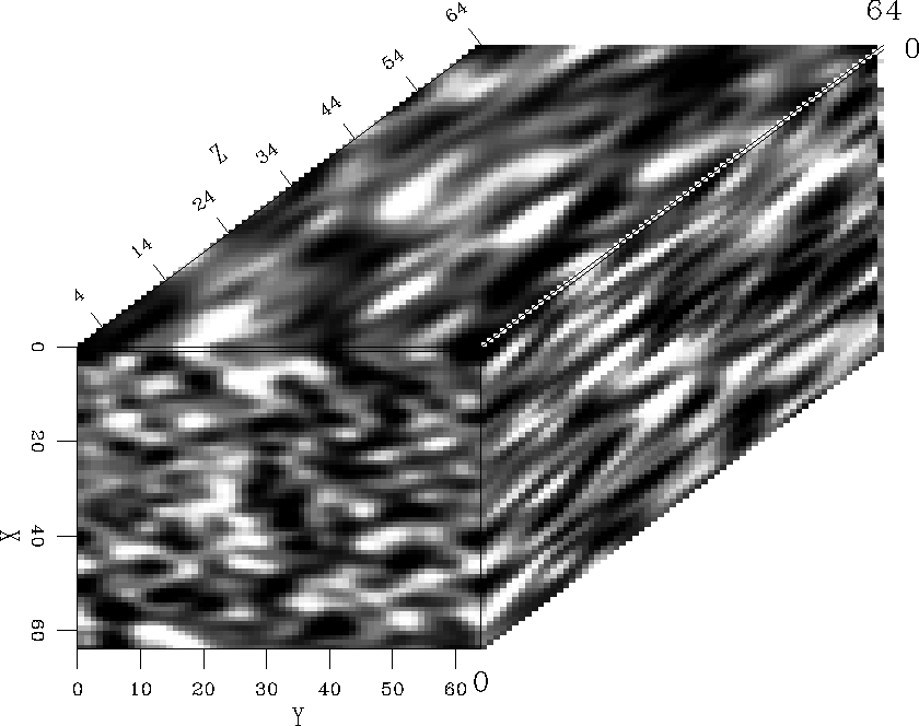
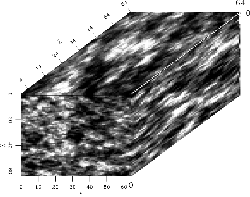
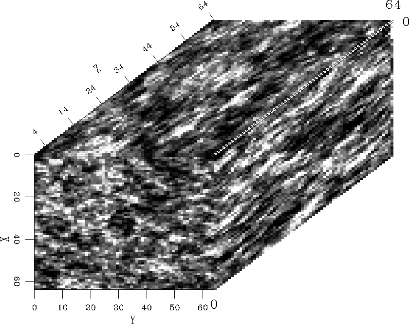
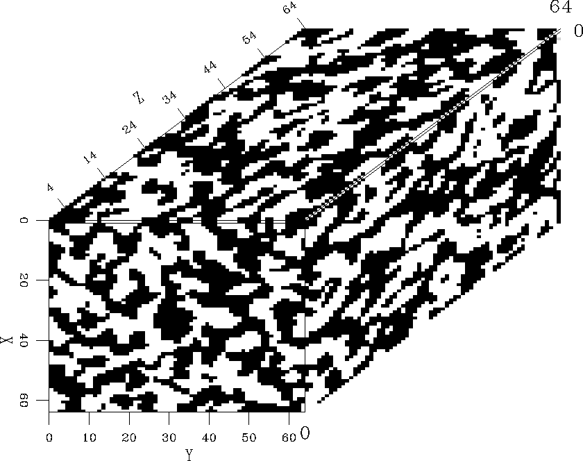
I show three different realizations of an anisotropic model with different aspect ratios along the three coordinate axes. The model is a 64 points cube with characteristic scales a_x=15, a_y=25, and a_z=35. The media are characterized by Gaussian, exponential, and van karman autocorrelation functions, respectively. We notice the increase in model roughness as we move from the Gaussian medium to the exponential field (i.e, $\nu=.5$) and then to the von Karman field with $\nu=.2$.

In the physical world, these fields may represent media at different scales varying from the microscopic to the megascopic.

Modeling seismic impedances

Seismic impedances have frequently been modeled as a Markov process. Godfrey et. al. (1980) modeled impedance as a special type of Markov chain, one that is constrained to have a purely exponential correlation function. They tested their method on three actual logs and compared the autocorrelation function to a best fit exponential curve. Apart from a small geologic noise component at the origin, their results showed excellent agreement between the theoretical exponential and the actual autocorrelation on two of the well logs they considered. For large lags, the actual correlation function had exponential behavior similar to that of the theoretical curve, but all data points fell below the synthetic curve showing a faster decay rate. The behavior of the autocorrelation could very well be interpreted as related to a rougher distribution than that predicted by the exponential correlation. A von Karman correlation function with a Hurst number smaller than 0.5 would have given a better fit to the autocorrelation of the impedance series. The autocorrelation of the impedance function provides information on the depositional pattern in the sedimentary column i.e, cyclic or transitional ().

Figure imped shows a comparison of one-dimensional random sequences that simulate synthetic impedances with von Karman correlation functions of varying fractal dimensions (i.e., Hurst number $\nu$). Again the smaller the value of $\nu$, the rougher the sequence. The impedance with exponential correlation seems smooth compared to the ones generated from autocorrelation functions with values of $\nu$ lower than 0.5.

impedheight=3.5in,width=6.inSynthetic random sequences simulating acoustic impedances with von Karman autocorrelation for varying Hurst number $\nu$.

GENERATING TWO-STATE MODELS

In the geophysical world we often deal with heterogeneous media whose inhomogeneities are caused by the presence of two different types of material with different mechanical properties. A typical example is the case of a stratified formation of shale embedded in sandstone. In fluid flow and reservoir engineering problems, the rock samples are generally composed of a matrix and pore space. Continuously random fields are therefore inadequate to describe randomness in similar settings. I seek to describe a random field in which the medium can be represented as a two-state model. This new field is called a binary field and the process of deriving the binary field from the continuous field is called ``binarization'' (). The problem is to relate the statistics of the binary field to those of the continuous field. Holliger et al. (1993) gave a brief description of their mapped two-dimensional binary field which I apply in a straightforward generalization to the three-dimensional problem.

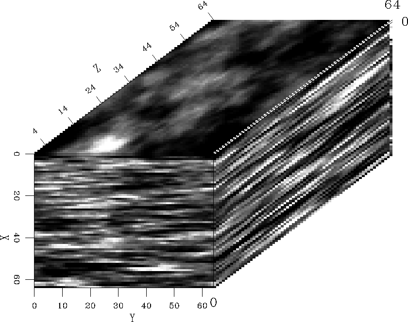
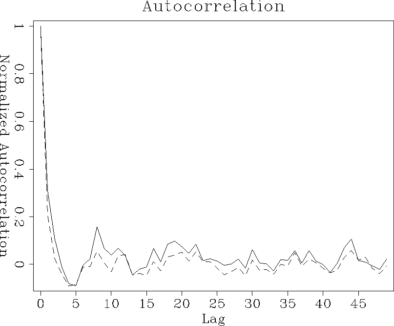
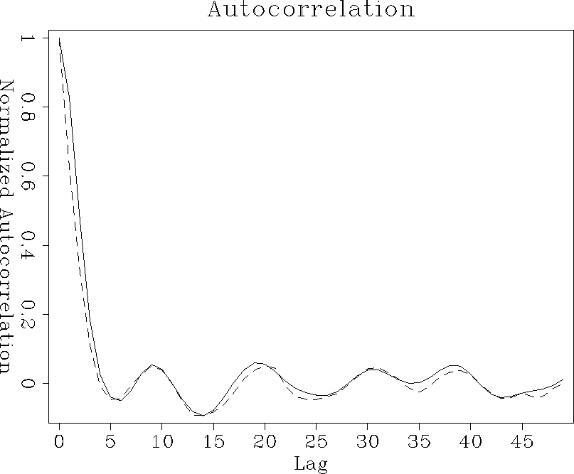
To illustrate the effects of ``binarizing'' a continuous field, let's consider two examples of random fields with Gaussian and exponential autocorrelation functions, respectively. In the first example I simulate a randomly-stratified medium. The second example is a realization of a random medium with statistically isotropic homogeneous inclusions. I like to analyze the change in the medium properties by comparing the autocorrelation function of the distribution before and after ``binarization''. For better observation, I limit the analysis to the study of the correlation function along one axis, i.e, in the x-direction.

Figure auto-expo shows the averaged 1-D correlation function along the x-axis for the randomly layered medium. The solid curve displays the autocorrelation of the continuous field; the dashed one represents the autocorrelation of the ``binary'' field. The two functions are noticeably different from one another; the slope near the origin is greatly increased after ``binarization'' indicating a rougher distribution compared to the continuous case. Figure auto-gauss shows the same observations for the isotropic random field with Gaussian autocorrelation; again the roughness of the field has increased as indicated by the steepening in the slope of the autocorrelation.

 

layered
Figure 4 Synthetic continuous random field with apparent layering and Gaussian autocorrelation; a_x=5, a_y=80, a_z=80.

 

lay-bin
Figure 5 Synthetic binary field derived from the continuous realization of a layered random field with Gaussian autocorrelation.

 

isotropic
Figure 6 Synthetic continuous random field with isotropic Gaussian autocorrelation function; a_x=15, a_y=15, a_z=15.

 

iso-bin
Figure 7 Synthetic binary field derived from the continuous realization of a random field with Gaussian autocorrelation.

 

auto-expo
Figure 8 Autocorrelation functions of the continuous (solid lines) and binary (dashed lines) fields for the layered random medium with exponential correlation.

 

auto-gauss
Figure 9 Autocorrelation functions of the continuous (solid lines) and binary (dashed lines) fields for the isotropic random medium with Gaussian correlation

CONCLUSIONS

In this initial study I have tackled the forward problem for modeling anisotropic fractal media using second-order statistics. The method has close analogy with the two-dimensional Goff and Jordan model for seafloor morphology. The generation of synthetic models is done in the Fourier domain and the algorithms are similar for the one- two- and three-dimensional problems. The von Karman functions are presented as a generalization of the exponential correlation function associated with the Markov process in modeling seismic impedances. The von Karman functions can be used for better description of statistic lithology of stratigraphic columns and understanding their depositional pattern. I have also computed a two-state model (i.e., rock/pore or sandstone/shale) by mapping the random field from continuous realizations into a binary field. Comparisons of the autocorrelation functions of the continuous and binary fields show that the fractal dimension (i.e, the roughness of the medium) increases through the ``binarization'' process.

FUTURE WORK

Future goals of this effort will be to formulate the inverse problem for estimating the characteristic parameters of the anisotropic fractal medium, i.e, aspect ratios of anisotropy, and Hausdorff (fractal) dimension. The technique of deriving the binary field from the continuous random field should be extended to simulate M-state models, where M is the number of states or rocks composing an impedance well-log.

I also need to test the method on actual well-log data and demonstrate a better fit with von Karman correlation functions compared to the exponential fit. This would would be the first application of the inverse problem. Two and three dimensional problems can find application in the field of wave scattering and diffraction and in fluid flow problems.

A von Karman covariance function

Equation (4) in the text represents the autocovariance of a random medium of fractal nature. The power spectrum of the field corresponds to the Fourier transform of its covariance function:  

$$P(k)=\int_{-\infty}^{+\infty}\int_{-\infty}^{+\infty}\int_{-\infty}^{+\infty} C(r)e^{-ik\cdot r} d^3r \\ end{displaymath}$$ (12)

Using the N-dimensional Hankel transform (), the covariance function and its Fourier transform can be related as follows:  

$$p(k)=(2\pi)^{N/2}k^{-N/2+1}\int_{0}^{\infty} r^{N/2}J_{N/2-1}(rk)C(r)dr \\ end{displaymath}$$ (13)

 

$$C(r)=(2\pi)^{-N/2}r^{-N/2+1}\int_{0}^{\infty} k^{N/2}J_{N/2-1}(rk)P(k)dk \\ end{displaymath}$$ (14)

where J_N/2-1 is the Bessel function of order N/2-1.
The covariance C(r) in (3) is specified in terms of the function:  

$$G_\nu (r)=r^\nu K_\nu (r) \hspace{.3in} 0\leq r < \infty \hspace{.3in} \nu \in [0,1]\\ end{displaymath}$$ (15)

whose Hankel transform pair has been derived by Lord (1954):  

$$P(k)=\frac {\Gamma{(\nu +N/2)}} {2^{1-N-\nu}\pi{^N/2}} {(1+k^2)}^{-\nu-N/2} \\ end{displaymath}$$ (16)

where $\Gamma$ is the gamma function defined as:  

$$\Gamma (z)= \int_{0}^{\infty} t^{z-1}e^{-t} dt \\ end{displaymath}$$ (17)

Finally if we normalize $G_\nu (r)$ by $G_\nu (0)$ as in Goff and Jordan (1988), we obtain, for the three-dimensional case, the power spectrum of the field whose covariance is defined by (4):  

$$P(k)=4\pi\nu H^2 {(1+k^2)}^{(-\nu-3/2)} \\ end{displaymath}$$ (18)

[SEP,random]