

![[*]](http://sepwww.stanford.edu/latex2html/prev_gr.gif)


ABSTRACTAmong the suite of prestack imaging methods available, profile imaging method is the most suited for providing wave-theoretical angle-dependent reflectivity estimates. In this study, we tested profile imaging method for its ability to preserve angle-dependent reflectivity on the image. A synthetic shot gather was generated by an elastic finite-difference modeling code (Karrenbach, 1992) for a shale and gas-sand model (Ostrander, 1982). The profile imaging was performed with phase-shift and finite-difference approaches. |
During the past decade, the use of AVO (amplitude versus offset) analysis in petroleum exploration has become increasingly common. Even though the objective of AVO analysis is to observe an anomalous angle-dependent reflectivity behavior of a reflector, the name amplitude versus offset was chosen because most of the amplitude analysis is done in the common midpoint domain.
Knowing the incidence angle at a reflector and the corresponding reflectivity, we can analyze the properties of the reflector more correctly. Thus, angle-dependent reflectivity analysis can provide more accurate information about the reflector than AVO analysis in common midpoint domain.
One possible approach for obtaining angle-dependent reflectivity is to use profile imaging. Since profile imaging theoretically provides a reflectivity map for the subsurface image, we can construct angle-dependent reflectivity panels with the help of additional information, namely, the incidence angle of the wavefield at a given subsurface point.
In this study, we test the profile imaging method on a synthetic dataset to observe its ability to preserve the angle-dependent reflectivity effect.
REVIEW OF PROFILE IMAGING After removal of multiple reflections, the model for the primary reflection data of a shot profile can be formulated (Berkhout, 1985) as
| (1) |
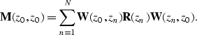 |
(2) |
In equation (1) the source vector ![]() and the measurement vector
and the measurement vector ![]() refer to a single seismic experiment at the surface z=z0.
In equation (2) the propagation matrices
refer to a single seismic experiment at the surface z=z0.
In equation (2) the propagation matrices ![]() and
and ![]() quantify the full propagation effects
(upward and downward, respectively) between depth levels z0 and zn;
the reflection matrix
quantify the full propagation effects
(upward and downward, respectively) between depth levels z0 and zn;
the reflection matrix ![]() defines the elastic angle-dependent
reflection properties caused by inhomogeneities at a depth level zn
and by the source wavefield
defines the elastic angle-dependent
reflection properties caused by inhomogeneities at a depth level zn
and by the source wavefield ![]() .All vectors and matrices refer to one temporal Fourier component.
.All vectors and matrices refer to one temporal Fourier component.
For a more clear explanation, we can rewrite equation (1) in terms of the series
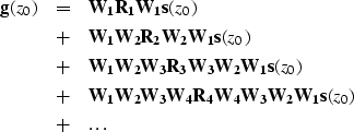 |
||
| (3) |
The purpose of profile imaging is
to recover angle-dependent reflectivity ![]() from
from ![]() and
and ![]() ,assuming that we know the subsurface velocity.
From the velocity field we can compute the
propagation operator
,assuming that we know the subsurface velocity.
From the velocity field we can compute the
propagation operator ![]() .
.
First, we remove the propagation effect ![]() from the received field by multiplying
both sides of equation (3) by
from the received field by multiplying
both sides of equation (3) by ![]() , which yields
, which yields
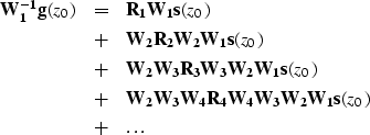 |
||
| (4) |
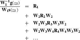 |
||
| (5) |
The procedure requires the inverse of the propagation operator,
![]() . In practical seismic migration, however,
the following approximation is commonly assumed:
. In practical seismic migration, however,
the following approximation is commonly assumed:
| (6) |
SYNTHETIC MODELING
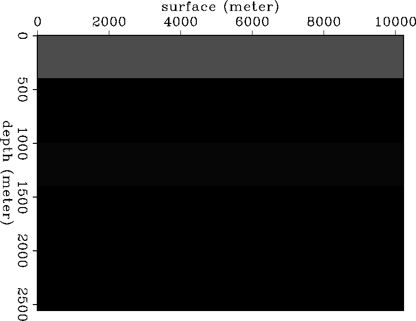
In order to test the profile imaging, we generate a synthetic model. For our test, we used a four-layer model containing water, shale, and gas sandstone, as shown in Figure velmodel. The elastic parameters of shale and gas sandstone were taken from Ostrander's (1982) paper, which reported very interesting results for AVO effects. The model parameters are given in this table:
| layer | thickness | velocity | density | Poisson's ratio |
| water | 400 m | 1500 m/s | 1.0 gm/cc | 0.0 |
| shale | 600 m | 3048 m/s | 2.4 gm/cc | 0.4 |
| gas sand | 400 m | 2439 m/s | 2.14 gm/cc | 0.1 |
| shale | 1160 m | 3048 m/s | 2.4 gm/cc | 0.4 |
 |
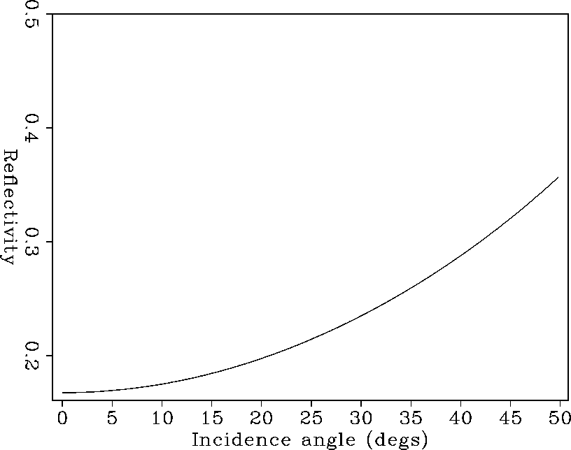
The theoretical angle-dependent reflectivity behavior of the second reflector, shown in Figure rflcoeff, was calculated with Zoeppritz equations.
 |
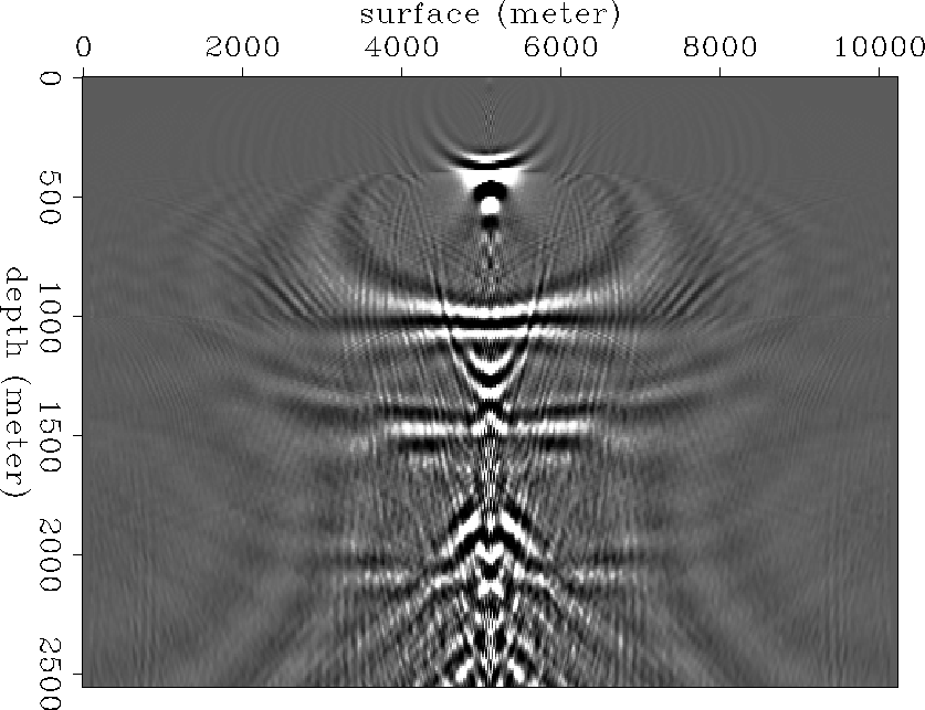
To generate a synthetic shot gather, we used an elastic FDM code (Karrenbach,1992). The resulting pressure wavefield appears in Figure shot-gather. The wavefield shown in Figure shot-gather is the pressure wavefield.
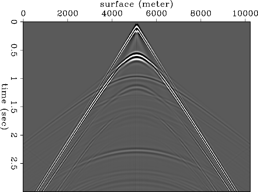 |
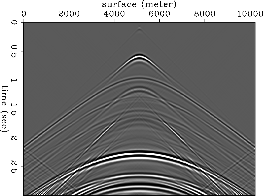
Figure shot-gather does not show any AVO effect for the reflection from the top of the gas-sand. This is because of the effect of geometrical spreading and also because the relative amplitude of this reflection with respect to the other reflections is small. Since the propagation operator in equation (6) does not incorporate such amplitude variation into the propagation, we need to scale up the later time events before imaging. We used RMS (root mean square) velocity to compensate for the geometrical spreading effect and applied a high-dip cut filter to remove strong water-bottom reflections. Figure shot-scale shows the shot gather after this preprocessing. It shows some AVO effect for the reflections from the top of the gas sandstone even though it is very small (Figure shot-scale).
 |
PROFILE IMAGING
Phase-shift approach Since the model we used has a 1-D structure, we were able to use the phase-shift approach (Gazdag, 1978), which is the most accurate for such a velocity model. Figure gaz-img shows the image after profile imaging using the phase shift propagation operator.
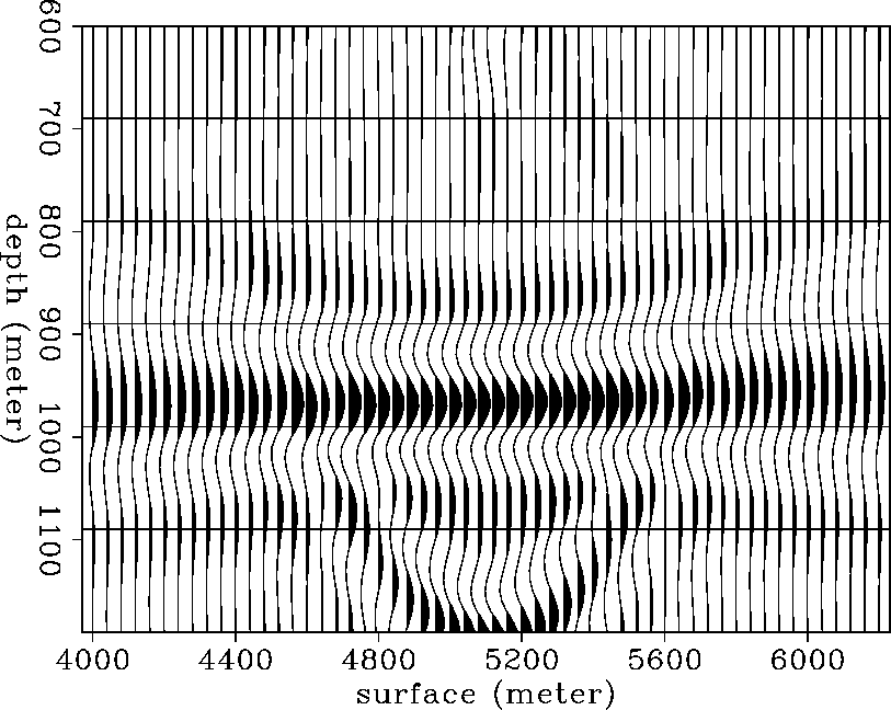
In order to show the amplitude behavior more clearly, the top of the gas sand was windowed out and plotted in wiggle form (Figure wgaz-img). The recovered image is positioned correctly in space but the amplitude of reflection coefficient does not show the angle-dependent reflectivity effect clearly.
 |
 |
Finite-Difference approach For the same model, we applied a finite-difference approach (Claerbout, 1985), the most popular extrapolation scheme. To increase the accuracy of the finite-difference extrapolation, we used Lee and Suh's (1985) optimized coefficient, which is accurate up to 65 degrees.
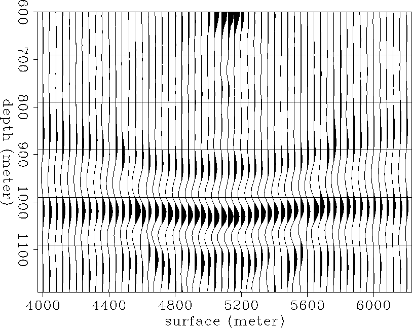
Figure fdm-img shows the image after profile imaging using the finite-difference operator for propagation. In order to show the amplitude behavior more clearly, the top of the gas sand was windowed out and plotted in wiggle form (Figure wfdm-img). The recovered image is positioned correctly in space, but the amplitude of the reflection coefficient does not show the angle-dependent reflectivity effect clearly.
 |
 |
DISCUSSION The results of testing the ability of recovering angle-dependent reflectivity by profile imaging show limited success. Even for a simple model, profile imaging does not recover the angle-dependent reflectivity in the image. One possible reason for the failure might be the propagation operator we used. The propagation operator used in the profile imaging is a depth-extrapolation operator, which does not take into account the geometrical spreading effect and the transmission factor. The correction for the geometrical spreading effect is valid only for the upcoming wave field.
In order to recover the angle-dependent reflectivity correctly, we need to have an accurate upcoming and downgoing wavefield at each depth level. To achieve this goal, we require an extrapolation operator that takes into account both the transmission loss factor and the geometrical spreading. The time-extrapolation algorithm has such characteristics, but is too expensive to use for shot-profile imaging.