Toward an exact adjoint:
semicircle versus hyperbola

Jun Ji

Author has no known email address

ABSTRACT

The correctness of an adjoint operator entirely depends on the correctness of the corresponding forward modeling operator. In migration, the input-oriented algorithm implies more correct forward modeling than the output-oriented algorithm does. One big difference between the two algorithms is the domain of interpolation, and this is one of the major sources of migration artifacts. Whereas the input-oriented algorithm requires interpolation in the model space, the output-oriented algorithm requires interpolation in the data space. For Kirchhoff migration, the method of semicircle superposition and the method of hyperbola summation correspond to the input-oriented and output-oriented algorithms, respectively. The same analogy can be applied to Stolt migration. Levin (1994) suggested the input-oriented algorithm that is the counterpart to the output-oriented algorithm suggested by the SEP ``in-time" group (Popovici et al., 1993; Lin et al.,1993; Blondel and Muir, 1993)

An adjoint operator to a forward modeling operator is often a good processing operator for estimating approximate model parameters from data that are assumed to follow the presumed forward modeling operator (Claerbout, 1992). Two of the most widely used approaches for finding the adjoint operator can be explained in three steps as follows:

• Approach 1

  1.

  Formulate the forward operator in the continuous sense.

  2.

  Write down the adjoint operator to the continuous forward operator.

  3.

  Discretize the continuous adjoint operator.

• Approach 2

  1.

  Formulate the forward operator in the continuous sense.

  2.

  Discretize the continuous forward operator.

  3.

  Take the Hermitian adjoint of this discrete operator.

The difference between the adjoint operators acquired by theese two approaches is a weighting factor. The adjoint operator obtained by the first approach has a weighting factor that is the Jacobian, but the one found by the second approach does not have it. The Jacobian appears while finding the adjoint operator in the continuous sense.

With each approach, there are two types of adjoint operators that depends on the discretizing space. While the discretization of an operator along the data space results in an algorithm that requires looping over the data space, the discretization of an operator along the model space results in an algorithm that requires looping over model space. An example is hyperbolic summation versus semicircular superposition in the Kirchhoff migration.

Even though the discretization of an operator along the data space is more correct than the other approach in simulating the real experiment, we are used to discretizing along the model space because of the ease of numerical implementation. Claerbout has reported, however, some advantages of the algorithm that uses looping over model space in NMO (Claebout, 1990) and velocity scanning (Claebout, 1989).

This paper compares the two algorithms that require looping over the data space and over the model space, in terms of the implied forward modeling operator and tests both algorithms with and without Jacobian in Kirchhoff migration and Stolt migration

FORWARD MODELING Even though the model space of the real world, ${\bf m}$,is continuous space, the data, ${\bf d}$,acquired are usually regularly discretized samples. In order to formulate a forward modeling operator that relates the continuous model space and the discrete data space, let us assume that ${\bf C}$ is the operator which relates continuous model space into continuous data space, and that ${\bf S}$ is a sampling operator. Then the entire forward modeling operator, ${\bf L}$,can be obtained by cascading both operators, as follows:

$${\bf d} = {\bf L m} = {\bf S C m} .$$ (1)

Since the continuous operator, ${\bf C}$, cannot be expressed with an explicit matrix, I have used Figure frd-oprt to explain this operation in terms of an abstract matrix. In Figure frd-oprt the dotted line represents the discrete data space, and the solid line represents the continuous model space.

frd-oprtheight=2.in,width=3.in The shape of the forward modelling operator (${\bf L = S C }$). The dotted line represents the discrete data space, and the solid line represents the continuous model space. Notice that the operator ${\bf L}$ is continuous in the model space and discrete in the data space.

There are two possible adjoint operators to the forward operator shown in equation (1). One case is when we assume the forward operator to be two cascaded operators such as ${\bf S C}$.Then the adjoint operator has the form like ${\bf C^T S^T}$.Here, ${\bf S^T}$ is a simple transposed matrix of ${\bf S}$,but ${\bf C^T}$ is not a simple transposed matrix because an adjoint operator in a continuous domain cannot be straightforwardly defined by transposing a corresponding matrix (we simply do not have the matrix). Instead another equivalent property can be used for dot-product definition (Claerbout, 1992); Jedlicka (1989) suggested the Euclidean norms. If we find ${\bf C^T}$ with respect to the Euclidean norms, the Jacobian appears in the process of variable substitution.

The other case is when we assume the forward operator to be a whole operator like ${\bf L}$.Then the adjoint operator has a form like ${\bf L^T}$. Even though this adjoint cannot be shown in an explicit matrix form because the model space is continuous (Figure frd-oprt), we can implement this easily by looping over the data space or, in other words, using the input-oriented algorithm.

Since the operators ${\bf S}$ and ${\bf C}$ are not commutative,

$${\bf S C} \ne {\bf C S},$$

the order of the two operators is very important in defining the forward modeling operator.

Defining our operator, ${\bf L}$,to have the form of ${\bf C S}$ instead of ${\bf S C}$,results in a different forward modeling operator,

$${\bf d} = {\bf L m} = {\bf C S m} .$$ (2)

This equation implies that the model space is sampled before we apply the forward operator, which is not correct. Figure frd-oprt-con explains this operation in terms of an abstract matrix.

Again we have two possible adjoint operators to the forward operator shown in equation (2), which can be derived the same way as I explained before.

frd-oprt-conheight=2.in,width=3.in The shape of the forward modelling operator (${\bf L = C S}$). The dotted line represents the discrete model space, and the solid line represents the continuous data space. Notice that the operator ${\bf L}$ is continuous in the data space and discrete in the model space.

Even though the continuous forward operators implied by both equations (1) and (2) are same, the algorithms for corresponding adjoint operators are different. Equation (1) leads us to the input-oriented algorithm, equation (2) to the output-oriented algorithm. In SEP-65 Claerbout (1989) reported differences between the two algorithms in velocity scanning. In the following two sections, I compare the two formulations for the Kirchhoff and Stolt migrations.

KIRCHHOFF MODELING AND MIGRATION The simplest zero-offset Kirchhoff modeling and migration algorithm connects the data space and the model space using the relation between travel time and distance

$$t^2 = {( x^2 + z^2 ) \over v^2} ,$$ (3)

where v is velocity, t is time, and x and z are surface and depth, respectively.

If we assume the forward modeling has the form of equation (2), the corresponding Kirchhoff migration turns out to be the hyperbolic summation algorithm, which is especially popular these days. If we assume the forward modeling has the form of equation (1), however, the corresponding Kirchhoff migration turns out to be the semicircle-superposition, which is the classical approach (Schneider, 1971).

In the continuous formulation in both data and model spaces the hyperbolic and semicircle approaches produce same results. In the real world, however, the data space is discrete and the model space is also required to be discrete for the purpose of representation. Thus, the hyperbolic and semicircle approaches differ because equation (3) doesn't allow mapping from regularly discretized data space to model space and vice versa.

If we use the hyperbolic summation approach, the interpolation in the data space is required because a point in the model space never produces a hyperbola that fits into a regular grid in the data space. In contrast, if we use the semicircle-superposition approach, the interpolation in the model space is required for the same reason as with the hyperbola approach. If we recall the implied forward modeling operator, the semicircle approach seems to be the appropriate one. However, because of the efficiency of the hyperbolic approach in computer implementation, there has been a tendency to ignore the semicircle approach.

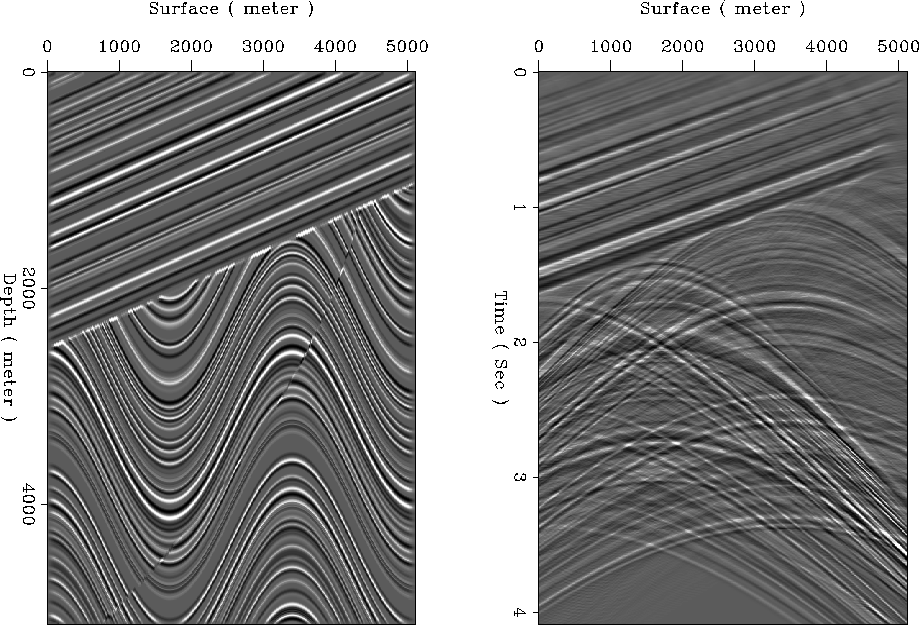
In order to investigate the possible advantage of the semicircle approach, I tested it and compared the results with those of the hyperbola approach. Figure kir-img-data shows a model and synthesized data. The model was generated using Claerbout's Sigmoid code with a fine sampling interval to avoid aliasing in the model space, and the data were generated using Claerbout's kirchslow algorithm. The sampling interval of the model used is so small that we can assume the modeled data is very close to the continuous situation.

 

kir-img-data
Figure 1 Synthesized subsurface image using Claerbout's Sigmoid (left) and modeled data using Claerbout's kirchslow algorithm (right).

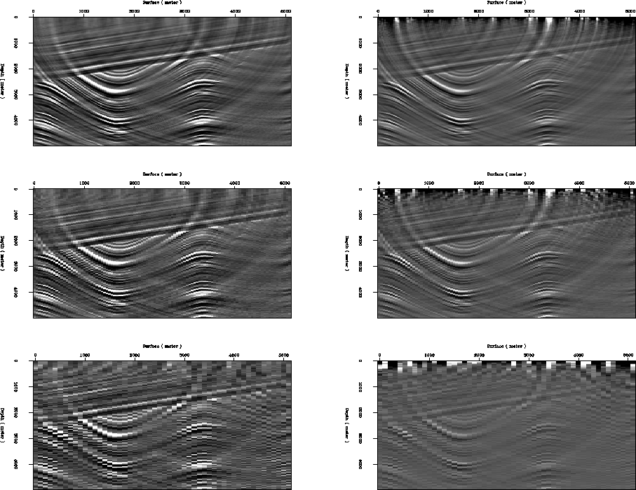
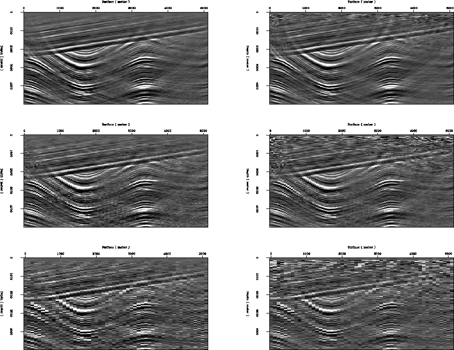
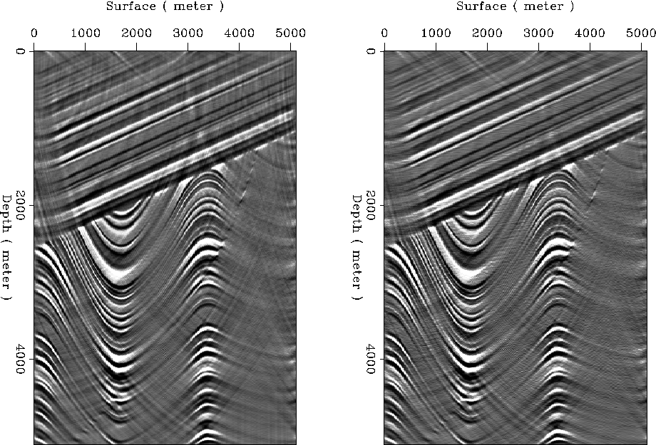
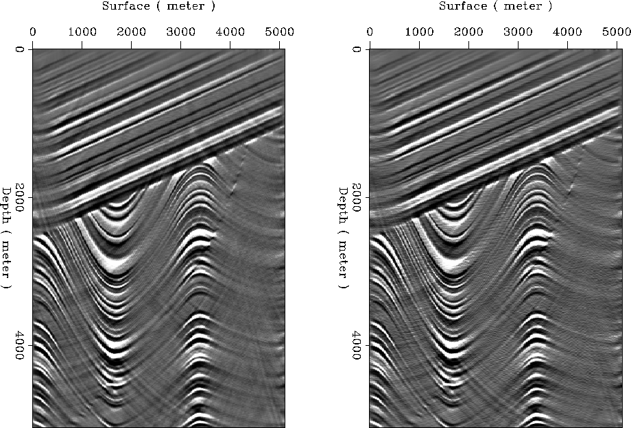
In order to simulate the discretized data along the surface, I subsampled the data (Figure kir-img-data) with sampling interval two, five, and ten times larger than the original one. First, the hyperbola summation was tested with and without the Jacobian for these subsampled data; the results appear in Figure kir-img-com-hp. In this case, the Jacobian does not seem to be helpful at all. Next the semicircle-superposition algorithm was tested with and without the Jacobian for the same subsampled data, and the results are shown in Figure kir-img-com-sc. Again the Jacobian does not seem to be helpful at all.

The results from both approaches are quite similar except for some artifacts in the image obtained by the hyperbolic summation. These artifacts are concentrated mainly in the portion where high dip events are located in the model space, which can be explained by the operator aliasing in the hyperbolic summation.

 

kir-img-com-hp
Figure 2 Migration results of Figure kir-img-data. The left images are the results of hyperbola summation without the Jacobian; the right images are with the Jacobian. To migrate the subsampled data, from the top every other, fifth, and tenth sample along the x direction is used.

 

kir-img-com-sc
Figure 3 Migration results of Figure kir-img-data. The left images are the results of semicircle-superposition without the Jacobian; the right images are with the Jacobian. To migrate the subsampled data, from the top every other, fifth, and tenth sample along the x direction is used.

STOLT MODELING AND MIGRATION The Stolt (1978) modeling and migration algorithm relates the data spectrum space and the model spectrum space using the dispersion relation

$${\omega^2 \over v^2} = ( k_x^2 + k_z^2 ),$$ (4)

where $\omega$ is temporal frequency and k_x and k_z are spatial wavenumbers.

In Stolt modeling and migration, unlike Kirchhoff methods, the interpolation is very important because the mapping from model and data is done in the spectrum domain. Recent SEP articles ( Popovici et al., 1993; Lin et al., 1993; Blondel and Muir, 1993) report on the testing of a Stolt migration and modeling method using the slow Fourier transform to reduce interpolation artifacts. Their algorithm implies the interpolation in the data space by slow Fourier transform along the irregularly located $\omega$,which is related to the regularly sampled in k_z. This method assumes that the forward modeling has the form of equation (2), and the corresponding Stolt migration turns out to be spectrum mapping following the hyperbolic equation.

As with the relation between the semicircle-superposition and hyperbolic-summation, there is an alternative to the slow Fourier transform along time axis. It is slow Fourier transform along the depth axis, as suggested by Levin (1994). This implies that the forward modeling has the form of equation (1), and the corresponding Stolt migration turns out to be spectrum mapping following the semicircle equation.

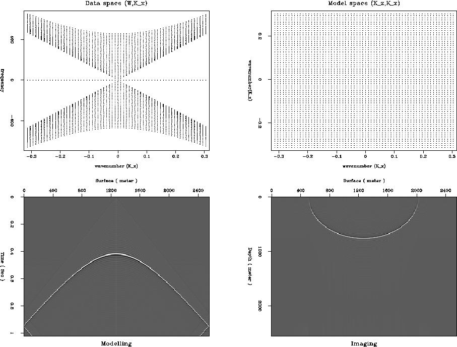
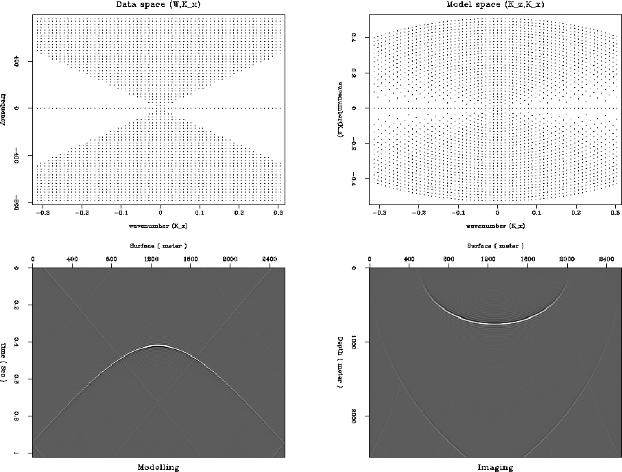
To show the spectrum mapping strategy in both approaches, each point in the model and data spectra are mapped and shown in Figures stolt-com2 and  stolt-com3, which also contain impulse responses. The impulse responses indicate that the interpolation in the data space shows fewer artifacts than the interpolation in the model space. However, the impulse response sometimes hides the defects of the operator, which is the case in these examples.

For a more accurate comparison, the migration operators of the both approaches were tested on the Sigmoid model of Figure kir-img-data; the results are shown in Figures stolt-sig-com-hp and  stolt-sig-com-sc. In these results, similar patterns of artifacts appear, and generally the input-orient algorithm produces a better image than the output-orient algorithm.

Unlike the Kirchhoff case, in this case, the Jacobian seems to help reduce the artifacts with both approaches (see Figures stolt-sig-com-hp and  stolt-sig-com-sc.)

 

stolt-com2
Figure 4 Stolt modelling and imaging regularly sampled for wavenumber and irregularly sampled for frequency.

 

stolt-com3
Figure 5 Stolt modelling and imaging regularly sampled for frequency and irregularly sampled for wavenumber.

 

stolt-sig-com-hp
Figure 6 Stolt imaging for the Sigmoid synthetic regularly sampled for wavenumber and irregularly sampled for frequency. The left is without the Jacobian; the right is with the Jacobian.

 

stolt-sig-com-sc
Figure 7 Stolt imaging for the Sigmoid synthetic regularly sampled for frequency and irregularly sampled for wavenumber. The left is without the Jacobian; the right is with the Jacobian.

The correctness of an adjoint operator depends entirely on the correctness of the corresponding forward modeling operator. In migration, the input-oriented algorithm implies more correct forward modeling than the output-oriented algorithm. One big difference between two algorithms is the domain of interpolation, which is one of the major sources of migration artifacts. The input-oriented algorithm requires interpolation in the model space, but the output-oriented algorithm requires interpolation in the data space. In both algorithms, the Jacobian may or may not appear according to the definition of the implied forward operators. The usefulness of the existence of the Jacobian is not yet clear. The tests seem to indicate that the Jacobian helps in Stolt migration but did not in Kirchhoff migration.

• Blondel, P., and Muir, F., 1993, Parallel computing exhumes slow Fourier transform: SEP-79, 265-268.

• Claerbout, J. F., 1990, Hyperbola tricks: SEP-65, 241-246.

• Claerbout, J. F., 1992, Earth Soundings Analysis: Processing versus Inversion: Blackwell Scientific Publications.

• Jedlicka, J., 1989, Velocity analysis by inversion: SEP-61, 41-68.

• Levin, A. S., 1994, Stolt without artifacts? - dropping the Jacobian: SEP-80, 513-532.

• Lin, J. Y., Teng, L., and Muir. F., 1993, Comparison of different interpolation methods for Stolt migration: SEP-79, 255-260.

• Ottolini, R., 1990, Pixel-precise transforms as dip filters: SEP-67, 51-56.

• Popovici, A. M., Blondel, P., and Muir, F., 1993, Interpolation in Stolt migration: SEP-79, 261-264.

• Schneider, W. A., 1971, Developments in seismic data processing and analysis (1968-1970): Geophysics 36, 1043-1073.

• Stolt, R. H., 1978, Migration by Fourier transform: Geophysics 43, 23-48.

The definition of an adjoint operator in a continuous domain cannot be done straightforwardly by transposing a corresponding matrix (we simply do not have the matrix). Instead another equivalent property is used for definition:

$$({\bf Cm,d}) = ({\bf m,C^Td})$$ (5)

This is the equation that is used for the dot product tests (Claerbout, 1985) If we want to apply an algorithm using Euclidean norms, then our operators should be adjoint with respect to the Euclidean norms.

The definition of the simplest Kirchhoff modeling operator ${\bf C}$ is

$${\bf d}(t,x) = \int_y {\bf m}(\sqrt{t^2 v^2-(x-y)^2},x-y) dy$$ (6)

Let us derive the adjoint operator ${\bf C^T}$:

$$\begin{eqnarray} ({\bf Cm,d}) & = & \int_x \int_t {\bf d}(t,x) dt dx \int_y {\bf... ...t \int_y dt dx dy {\bf d}(t,x) {\bf m}(\sqrt{t^2 v^2-(x-y)^2},x-y)\end{eqnarray}$$ (7) (8)

After substitution $z=\sqrt{t^2 v^2 -(x-y)^2}$ and dt = z /(t v²) dz, we obtain

$$\begin{eqnarray} ({\bf Cm,d}) & = & \int_y \int_z {\bf m}(z,x-y) dy dz \int_x {z... ...}{\bf d}({\sqrt{z^2+y^2}\over v},y-x) dx \\ & = & ({\bf m,C^T d})\end{eqnarray}$$ (9) (10) (11)

Finally we have the Kirchhoff migration operator ${\bf C^T}$ is

$${\bf m}(z,y) = \int_y {z \over t v^2}{\bf d}({\sqrt{z^2+y^2}\over v},y-x) dx$$ (12)