

![[*]](http://sepwww.stanford.edu/latex2html/prev_gr.gif)


ABSTRACTA method for computing first arrival traveltimes and amplitudes in a general two-dimensional (2-D) velocity model is presented. The method is the result of merging two recently published ray tracing methods. The product is a very robust algorithm that is able to produce broadband wave phenomena, such as dispersion and wavelength dependent scattering. Its ability to produce broadband wave phenomena, is achieved by performing a wavelength-dependent smoothing of the velocity model across wavefronts. In the limit of high frequency, the method reduces to geometrical ray theory. The method is able to illuminate areas of large geometrical spreading where conventional ray tracing methods may give no arrivals. The method is tested on synthetic complex velocity models. |
Traditionally traveltime and amplitude calculations have been performed by ray tracing. Different ray tracing algorithms exist that are well known and well documented. They include Julian and Gubbins' ray bending, Dines and Lytle's shooting rays and Cervený's paraxial extrapolation. More recently, several new methods have appeared and are enjoying an increasing popularity. They include Vidale , Podvin and Lecomte , van Trier and Symes finite differences and Moser's shortest path rays.
This paper presents a review of two new ray tracing methods and explores some of the possibilities produced by their fusion. The first method is Lomax's waveray method for approximating broadband wave propagation through complex velocity structures. The second method was developed at the NORSAR institute in Norway by Vinje, Iversen and Gjøystdal . As will be shown later, both methods have their own advantages and drawbacks, but when they are fused, they interfere positively. The combined product produces a very robust method, which approximates broadband wave phenomena in complex velocity models.
The first two parts of this paper describe the basic characteristics of each method and their implementations. The paper also reviews some of the work done in the last two references listed above. In the last part, I discuss the combined method. Implementation issues and synthetic examples are shown.
LOMAX'S WAVERAYS
Two basic ideas characterize Lomax's method: (1) it does a wavelength-dependent velocity smoothing and (2) it uses Huygen's principle to track the motion of narrow-band wavefronts at a number of center frequencies. Narrow-band wavefronts are defined as surfaces (lines in 2-D) of constant phase or traveltime in a narrow-band ``wavefield''. As these narrow-band wavefronts propagate with time they define a wavepath, which is frequency dependent. The wavelength-dependent smoothing of the velocity is done by averaging with a Gaussian weighting curve. The smoothing is done along the wavefronts. The final result; i.e, the broadband wavefield, is constructed by summing the results of independent narrow-band wavefields at many center frequencies.
Three important advantages of using Lomax's waveray over conventional ray tracing methods are:
In Lomax , the author approximates the narrow-band wavefronts at any time by a plane wavefront (see Figure lomax1). This approximation requires that the radius of curvature of the wavefront be large relative to a wavelength. A better approximation to the wavefronts could probably be obtained using a parabolic approximation. For the sake of computational time, plane wavefronts are used.
Before considering the details of the waveray technique, two points need to be emphasized. First, Lomax points out, ``it is the wavelength dependent smoothing that makes the waveray method a broadband wave propagation technique, and distinguishes it from the high frequency ray methods.'' Second, there are no equations that give the waveray method a theoretical basis. Its support comes from the fact that it reproduces high-frequency ray propagation and produces a good approximation of broadband wave phenomena.
lomax1width=3.in.Waveray wavepath and
wavelength-dependent velocity smoothing at point ![]() Adapted from Lomax (1994).
Adapted from Lomax (1994).
Waveray implementation
In the waveray method, the wavelength-dependent
averaging of the velocity is done dynamically as a function
of the position and orientation of the plane wavefronts.
The velocity
averaging is done using a Gaussian weight curve, centered at the wavepath
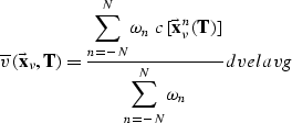
location (see Figure lomax1). Equation velavg expresses the
wavelength averaged velocity ![]() at a point
(
at a point
(![]() ) for a wave period
) for a wave period ![]() (),
(),
 |
(1) |
| (2) |
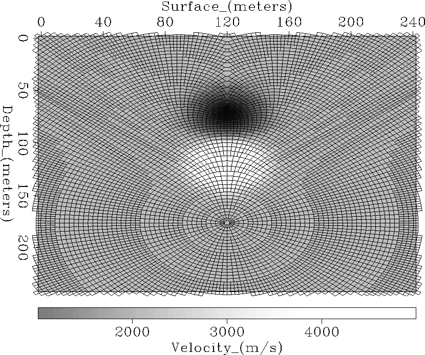
(![]() ) is the position along the
instantaneous straight wavefront given by the recursive relation
():
) is the position along the
instantaneous straight wavefront given by the recursive relation
():
| (3) |
The discrete representation of equation velavg is given by equation dvelavg:
 |
(4) |
| (5) |
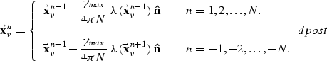 |
(6) |
These two equations are the discrete version of equation post, but,
the dependence on the wavelength has been made explicit.
Notice that the subscript ![]() of
of ![]() runs along the wavepath and the
superscript n runs along the wavefront.
runs along the wavepath and the
superscript n runs along the wavefront.
![]() specifies the largest distance in wavelengths along
the wavefront at which smoothing is applied.
specifies the largest distance in wavelengths along
the wavefront at which smoothing is applied.
The discrete equivalent of the Gaussian weight function is:
| (7) |
| (8) |
The motion of the waverays along the direction of propagation is expressed by the following equation:
| (9) |
lomax2width=3.in.Waveray wavepath calculation.
Huygen's principle is used to obtain the bending
![]() of the wavepath from points
of the wavepath from points ![]() and
and ![]() .Adapted from Lomax (1994).
.Adapted from Lomax (1994).
The change in direction of the waverays is approximated by the
difference in movement between the first control point on either
side of the wave location ![]() as shown in
Figure lomax2:
as shown in
Figure lomax2:
| (10) |
Finally, the half width parameter ![]() and the truncation
parameter
and the truncation
parameter ![]() are set at
are set at ![]() and
and ![]() , based on Lomax's
calibration. The number of control points N is set
proportional to the ratio
, based on Lomax's
calibration. The number of control points N is set
proportional to the ratio ![]() of the wave period over the
time step.
of the wave period over the
time step.
Figure lomaxsbs shows the significant differences between the waveray and ray methods. Notice how a high frequency ray is scattered by the small velocity anomaly, while the waveray's wavepath is little deflected. Note also, how the third ray (from right to left) is not perturbed by the low velocity anomaly, while the waveray wavepath is deflected. The wavelength-dependent velocity averaging smoothes out small velocity variations and causes the wavepath to be affected from velocity variations away from it.
lomaxsbs.Left frame shows a fan of high frequency ray paths. Right frame shows a fan of 12 Hz waveray wavepaths. The straight segments perpendicular to the waverays represent the instantaneous wavefronts. The velocity model is defined by two circular anomalies drawn in a homogeneous background. The black dot (located at 1000 m. by 1250 m. in depth) depicts a low velocity anomaly. The white circle a high one.
NORSAR WAVEFRONT CONSTRUCTION
The main idea behind the ``NORSAR'' method
is to compute ray parameters
along wavefronts instead of computing them from independently traced
rays, as conventional ray methods do. Wavefronts are defined as
isochron traveltime curves (lines in 2-D) from the source.
New wavefronts are constructed from previous ones, by ray tracing over
a time step. As wavefronts expand out, new rays are interpolated
between rays that go further apart than a predefined distance DSmax.
Figure norsar1 illustrates how wavefronts expand out, by ray
tracing from a time ![]() to a time
to a time ![]() . The
dashed line on Figure norsar1 represents the new
wavefront. The
solid dots represent the end points of the rays. The distance
between contiguous end points is checked against the predefined maximum
distance DSmax. If they are located further than
DSmax, a new point (empty dots) is interpolated.
. The
dashed line on Figure norsar1 represents the new
wavefront. The
solid dots represent the end points of the rays. The distance
between contiguous end points is checked against the predefined maximum
distance DSmax. If they are located further than
DSmax, a new point (empty dots) is interpolated.
The interpolation of these
new points over the wavefront is done using a vectorial
third order polynomial
![]() .The polynomial is evaluated as a function of the normalized
distance s between points
.The polynomial is evaluated as a function of the normalized
distance s between points ![]() and
and
![]() .Also a scalar third order polynomial is used to interpolate amplitude values
and the ray's angle of direction (see Vinje et. al. ).
.Also a scalar third order polynomial is used to interpolate amplitude values
and the ray's angle of direction (see Vinje et. al. ).
The key property of this procedure is that it produces a fairly constant density of rays over C1 models () (see Figure gauss-wv), illuminating zones with high geometrical spreading where conventional ray tracing have shadow zones.
norsar1.New wavefronts (dashed lines) are constructed from the previous wavefront (solid line), by ray tracing a fix number of time steps. New rays are interpolated between points on the wavefront that lay further than a predefined distance. Adapted from Vinje et. al. (1993).
Rays are eliminated if they go out of the model boundaries. They may also be eliminated if a wavefront crosses over itself, as shown on Figure norsar2. The ``self-crossing'' of the wavefronts may correspond to a caustic or to the intersection of rays from different parts of the model. Once again, as in the Lomax algorithm, for the sake of computational time and also of memory, a ``first arrival'' mode should be used. This first arrival mode removes all later arrivals. When the number of points in a wavefront becomes less than a certain value (e.g. 4 points), the algorithm stops.
Traveltimes and amplitudes are interpolated into a rectangular grid. Ray cells, defined as the area enclosed by a pair of contiguous rays and wavefronts, are checked for the presence of grid points (see Figure norsar3). Traveltimes at the receivers are estimated by computing the following quantities:
The traveltime at the receiver is then estimated to be:
| (11) |
norsar2.The new wavefront crosses itself. If only first arrivals are wanted, the points behind the crossing (points no. 7, 8, 9) are removed from the wavefront. Adapted from Vinje et. al. (1993).
In computing amplitudes,
the geometrical spreading factor ![]() ,gives the ratio between the amplitude of one wavefront to the next
one. R1, R2, r1 and r2 are shown on
Figure norsar4. The amplitude estimation at
the receivers is also obtained in this way, where the distances
d1 and d2 are used for R1 and R2.
,gives the ratio between the amplitude of one wavefront to the next
one. R1, R2, r1 and r2 are shown on
Figure norsar4. The amplitude estimation at
the receivers is also obtained in this way, where the distances
d1 and d2 are used for R1 and R2.
Figure gauss-wv shows an example of the Norsar method run over a highly contrasted velocity model. The velocity model is a pair of Gaussian bell curves. The distance between the peaks is 48 meters with a drop of 4 km/s in velocity.
norsar3.Traveltimes and amplitudes are found at receivers by interpolating within each ray cell. The ray cell is defined by Ray1 and Ray2, and by the new wavefront and the previous wavefront. Adapted from Vinje et. al. (1993).
A final point on Norsar's method is, as said by Vinje et. al. : ``the way the ray tracing between each wavefront is performed is irrelevant to the idea of the wavefront construction''. We notice that all along the discussion on the NORSAR method, ray tracing was kept as an abstract idea. With this in mind we proceed to merge the Lomax algorithm, as the ray tracing algorithm for the NORSAR method. Another advantage of the NORSAR method is that the estimation of ray parameters (as traveltimes, amplitudes, etc.) does not come from a posteriori interpolation between single, separate rays, but instead directly from previously constructed wavefronts.
norsar4.Amplitudes are computed from the previous wavefront. The geometrical spreading factor gives the ratio between the amplitude Ai at the previous wavefront and the new amplitude value Ai+1.
 |
![[*]](http://sepwww.stanford.edu/latex2html/movie.gif)


WAVERAYS AND WAVEFRONTS
The product of merging the two previously discussed ray tracing methods is sketched in the following pseudo-code:
1 		 Allocate memory for wavefronts and output
2 		 for each source
3 		 		 initialize
4 		 		 while number of points in wavefront > 4
5 		 		 		 propagate wavefront
6 		 		 		 check for self crossing
7 		 		 		 check for rays that go out of bounds
8 		 		 		 eliminate self crossing and outofbound rays
9 		 		 		 calculate amplitudes
10 		 		 		 gridding
11 		 		 		 interpolate new rays
12 		 		 		 movwavf
The algorithm defines the data structure ``cube'' at line 1. In it, the ray parameters are stored as wavefronts propagate.
		 struct heptagon {
		 		  struct point {
		 		 		    float x;
		 		 		    float z; } x0, x1;
		 		  float angle;
		 		  float ampl;
		 		  char cf; } *cube;
where:
The index ii runs over the points of a wavefront. Since there is no a priori way of determining how large can a wavefront grow over a velocity model, a predefined limit (nrmax) of cube elements is established at the beginning of the algorithm, which defines the total memory allocated for cube. In other words, nrmax is the maximum number of points that a wavefront can have. If the wavefront grows bigger than nrmax points the algorithm is stopped and an error message is produce indicating that a bigger value for nrmax should be used. This integer depends directly on the maximum allowed separation DSmax between two contiguous points in the wavefront. For the examples shown on Figure marm80-time through marm10-ampl, the program ran with a value of nrmax=1300. DSmax was set to 21 meters for those examples.
In the case that the algorithm is run in a ``all arrivals'' mode, which could be done by eliminating line 6 out of the algorithm, the number of crossing points on a wavefront could become considerably large. As the wavefronts crosses and crosses many times over itself, for a velocity model with strong variations (as for example the Marmousi model), the number of crossing points can easily reach the 6 digits figure. This translates directly into a bigger need of computer resources, in use of memory and time.
Subroutine initialize defines the initial wavefront. It assigns an initial amplitude and take-off angle to the points on the initial wavefront.
The propagate wavefront subroutine ray traces using Lomax's waverays. The waverays are traced starting at cube[ii].x0 with a take-off angle cube[ii].angle during one time step at a certain frequency. The time step and the frequency are user predefined.
Subroutine on line 6 checks for self crossed wavefronts and flags the points that belong to the inner crossed section of the wavefront.
Line 7 checks for points that fall out of boundaries, raising a flag. Notice from Figure gauss-wv that the rays cross over the boundaries of the model. This is done in order to obtain arrivals at the receivers that lie on the boundaries.
Subroutine at line 8 eliminates the points on a wavefront that are flagged for laying out of bounds or belong to self crossed wavefronts.
Subroutines on lines 9, 10 and 11 are implemented as previously explained for the NORSAR method on Figures norsar4, norsar3 and norsar1 respectively. On line 11 the number of rays that may be interpolated between any two contiguous rays, is given by the number of times the distance between the two rays is bigger than the maximum allowed distance DSmax.
Subroutine gridding is a very time consuming, due to the irregular distribution of the data in the model. First, the subroutine checks for receivers inside the ray cells of two contiguous wavefronts. If a receiver is found, the ray parameters are interpolated to it.
Subroutine movwavf prepares the structure cube for a new wavefront to be propagated. It takes as the new starting point the previous arriving point (cube[ii].x0 = cube[ii].x1).
Travel-times and amplitudes in the Marmousi model
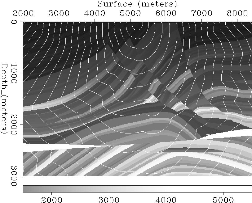
Figures marm80-time to marm10-ampl display the results of a simulation that used the combined method. The underlying subsurface structure is the Marmousi model (). A source was put at the surface, 5200 meters away from the left edge of the model, and the wavefronts were propagated until they crossed the boundaries of the model. Figure marm80-time shows the first-arrival traveltime contours calculated at a frequency of 80 Hz. Figure marm10-time shows the same experiment at a frequency of 10 Hz. Not much difference is apparent.
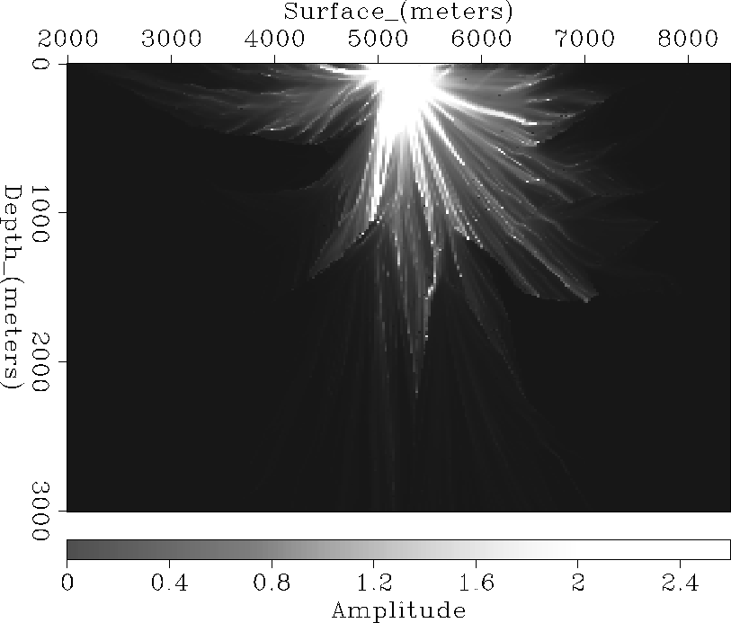
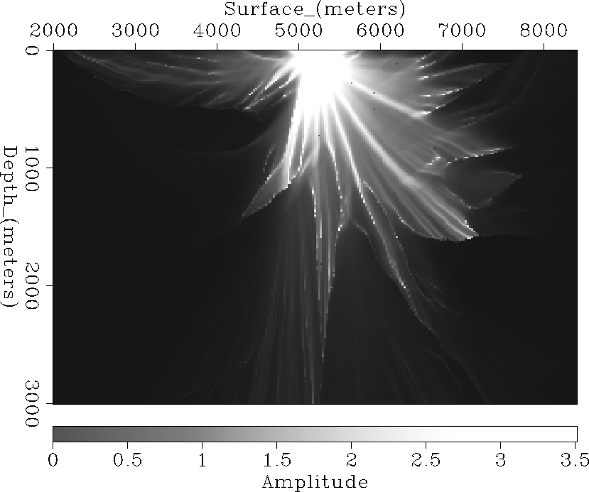
Figure marm80-ampl shows the amplitude estimates for the 80 Hz shot and Figure marm10-ampl shows the 10 Hz estimates. We see that more energy gets propagated down in the case of the low frequency, illuminating part of the high frequency shadow zones.
We have seen that the combined method accomplishes two important tasks, it can be used to compute first arrival traveltimes and amplitudes over any general velocity model and is it able to illuminate high frequency shadow zones.
For these experiments, the mesh of the model is re-sampled from the original model at 8 x 8 meters. The traveltime and amplitude outputs are placed in a mesh of 25 x 12.5 meters.
I have presented a review of two ray tracing methods. I have implemented both of them in a combined version. The method computes first arrival travel-times and amplitudes of seismic waves in complex 2-D velocity structures. The method uses a wavefront construction technique that produces a complete coverage of the medium by a fairly constant density of wavefronts and rays. Wavefronts are propagated using a wavelength-dependent smoothing ray tracing technique, called the waveray method, which leads to an increased stability of the ray paths relative to high frequency rays. Also, it gives a sensitivity to the rays to larger velocity anomalies that lay within a fraction of a wavelength of the ray path. The data (traveltimes and amplitudes) is computed on an irregular grid. As the wavefronts are constructed the data is interpolated into a regular grid.
The result is a very robust ray tracing method that is able to illuminate areas of large geometrical spreading zones where conventional ray tracing methods produce shadow zones. Portions of the diffracted energy is produced in these shadow zones.
Further work should be done on calibrating and testing the results produced by the combined method against other methods. Future work should be done on a formal derivation of the waveray method. Production of seismograms and a 3-D version are also sources of future work.
[SEP,GEOTLE,paper]
 |
 |
 |
 |