When is anti-aliasing needed in Kirchhoff migration?

Dimitri Bevc and David E. Lumley

Author has no known email address

ABSTRACT

We present criteria to determine when numerical integration of seismic data will incur operator aliasing. Although there are many ways to handle operator aliasing, they add expense to the computational task. This is especially true in three dimensions. A two-dimensional Kirchhoff migration example illustrates that the image zone of interest may not always require anti-aliasing and that considerable cost may be spared by not incorporating it.

In this paper we establish some rules of thumb as to when anti-aliasing is required in Kirchhoff migration. The same criteria are applicable to other processes such as DMO, velocity analysis, and wave-equation datuming.

There are many methods of handling operator aliasing. Gray  presented a method which involves low-pass filtering data traces with a variety of pass bands and then selecting input data from these sets of traces so that operator aliasing does not occur. Spatial trace interpolation is another method of dealing with the operator aliasing problem (). A draw back of the latter two methods is increased data volumes. Methods which limit the dip or aperture of the operator reduce aliasing without increasing the data volume, but at the expense of losing high-angle and wide-aperture information. An attractive and computationally efficient method of handling operator aliasing has been implemented by Claerbout . His dip-dependant triangular weighting method does not require multiple copies of the data to be kept in memory since the weights are generated and applied quickly on-the-fly.

Claerbout's triangular weighting method has been demonstrated to be efficient for 2-D (, ) and 3-D (, ) Kirchhoff time and depth migration. It has also been successfully adapted to DMO and wave-equation datuming operators (, ). Even though the triangular weighting method is very efficient, it still involves an extra computational cost. When the anti-aliased algorithm is implemented on the Connection Machine in FORTRAN 90, calls to an indirect addressing subroutine are required to extract data points from individual traces for summing into output locations. These calls turn out to be a bottleneck. In order to perform an anti-aliased migration with linear interpolation, six calls to the indirect addressing subroutine are required for each input trace location. For a 3-D migration, the indirect addressing is substantial.

Because this anti-aliasing is currently expensive on the CM5, we are motivated to determine when we can get away with not using it. While doing away with anti-aliasing is generally not a good idea, there are situations in which we may be able to live without it. For example, if we are running trial migrations to determine velocity models we may concentrate our efforts on portions of the data where operator aliasing is not a factor.

After developing criteria which link frequency and dip content of seismic data, we migrate a 2-D salt dome data set with and without anti-aliasing. The examples illustrate the effects of operator aliasing, how it can be ameliorated by aperture limitation and triangle weighted migration, and when anti-aliasing is unnecessary.

OPERATOR ALIASING Operator aliasing most often occurs when operator moveout across adjacent traces exceeds the time sampling rate. Cycle skips can occur when the operator is aliased. For a moveout curve with slope dt/dx, and data with a spatial Nyquist frequency of k_n, temporal frequencies above

$$\omega = {k_n\over{dt/dx}}$$

are aliased. In terms of the mesh spacing $\triangle x$ and operator slope dt/dx, operator aliasing will occur for all frequencies above f_op, where f_op is given by:

$$f_{op} \; = \; \frac{1}{2 (\frac{dt}{dx}) \triangle x}.$$ (1)

Defining the maximum stepout as $p = \delta x /\delta t$, the highest dip frequency in the data is given by

$$f_d \; = \; \frac{1}{2 p \triangle x}.$$ (2)

When the stepout is captured by the mesh spacing, $\delta x = \triangle x$, and $\delta t = \triangle t$, the highest unaliased dip frequency is equal to the Nyquist frequency $f_n = 1/2\triangle t$. In areas of economic interest, steep dips are often present in the data and f_d > f_n.

Anti-aliasing is called for when the frequency content of the data, f_s, falls between

$$\EQNLABEL{crit} f_{op} \; \leq \; f_s \; \leq \; f_d.$$ (3)

This situation is illustrated in Figure spectrum.

 

spectrum Figure 1 Operator aliasing, event dip, and frequency content of the data.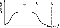

GULF OF MEXICO SALT DOME EXAMPLES In this section, we migrate a data set from the Gulf of Mexico to illustrate when anti-aliasing is not required. Migration is performed using an implementation of Claerbout's triangle weighted anti-aliasing scheme. Corresponding examples of standard Kirchhoff migration with and without angle limitation, are computed for comparison.

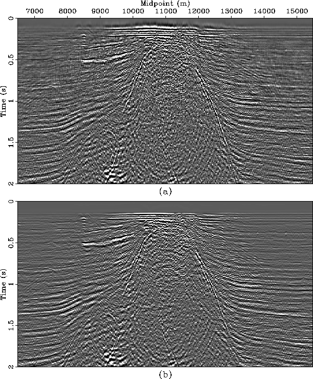
Anti-aliased migration The diffractions from the salt flanks are obvious in the near-offset section (Figure Gulfaaa) and can be seen to be spatially aliased. The data exhibit some overall speckling because of temporal aliasing. This temporal aliasing is due to recording or processing which was performed on the original data before it arrived at SEP. The anti-aliased migration is displayed in Figure Gulfaab. The salt flanks are nicely imaged and there is no evidence of operator aliasing. There are some artifacts due to the temporal aliasing: temporal aliasing is a different phenomena than operator aliasing and cannot be ameliorated by modifying the operator.

 

Gulfaa
Figure 2 (a) Near-offset section from the Gulf of Mexico. (b) Kirchhoff migration with triangle weighted anti-aliasing.

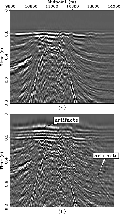
Aliased migration In Figure Gulfapera the data are migrated without triangular weighting. The effect of operator aliasing is most evident in the seafloor arrivals. We see precursors to the actual event. The top of the salt dome (earlier than t = 0.6 s) is poorly imaged and there is more overall speckling than in Figure Gulfaab, suggesting that the effects of data aliasing are compounded by operator aliasing. Other prominent operator aliasing artifacts are seen at about midpoints 13000 to 14000 and time 0.6 s to 0.9 s as cross-cutting dipping events. Figure Zoom2 is a comparison of the anti-aliased migration and the aliased migration (Figure Zoom2a is a closeup of Figure Gulfaab, and Figure Zoom2b is a closeup of Figure Gulfapera). The seafloor precursor artifacts before t=0.18 s and the cross-cutting dipping event artifacts are marked.

The operator aliasing has been somewhat contained by limiting the migration aperture to $45^\circ$ in Figure Gulfaperb; however, the seafloor event still has a precursor, the top of the salt dome is still poorly imaged, and there is more coherent noise than in Figure Gulfaab.

 

Gulfaper
Figure 3 (a) Kirchhoff migration without any aperture limitation or anti-aliasing. The effect of operator aliasing is noticeable at the seafloor where migration velocity is slow and where there is significant operator dip. At later times, the migration velocity is fast and there is not much operator dip, so there is no operator aliasing. (b) Kirchhoff migration of Gulf of Mexico data with $45^\circ$ aperture limitation. Limiting the aperture reduces some, but not all, of the operator aliasing at the seafloor.

 

Zoom2
Figure 4 Close up of (a) the anti-aliased migration, and (b) the standard Kirchhoff migration without anti-aliasing. The seafloor operator aliasing artifacts and the dipping artifacts are marked.

Anti-aliasing is not needed to image the salt flank The interesting thing about the images migrated without anti-aliasing is that in all cases the salt flank is nicely imaged at late times. This is because in this region the migration velocity is fast and the operator does not have much dip, so that f_op > f_s and operator aliasing is not a problem. At earlier times, the migration velocity is lower and the operator has significant dip so that f_op < f_s and operator aliasing is a problem.

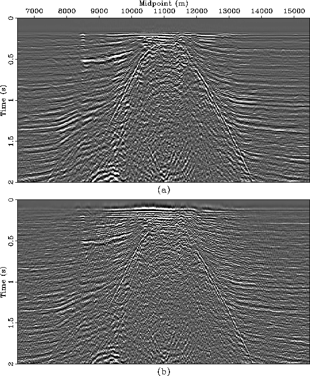
Migration with low velocity In Figure Miglow the data have been deliberately migrated with an unrealistic low velocity of 1000 m/s in order to confirm that operator aliasing will occur when the criteria of equation crit are met. In these examples f_op < f_s so that the operator is aliased. The diffraction from the salt flank is much better imaged in the anti-aliased migration (Figure Miglowa) than in the aliased migration (Figure Miglowb). All of the same operator aliasing artifacts that were visible at early times in Figure Gulfaa are still present, but now the events at late times also suffer. The right hand diffraction in Figure Miglowb is weaker and less continuous than the anti-aliased diffraction in Figure Miglowa. Some of the diffractions on the left side of Figure Miglowb are completely lost in the aliased migration.

 

Miglow
Figure 5 Kirchhoff migration of Gulf of Mexico data with an unrealistically low velocity: (a) with anti-aliasing, and (b) without anti-aliasing.

CONCLUSIONS We have presented a simple inequality which can be used to determine whether operator aliasing is a factor in Kirchhoff migration. The same criteria can be used for DMO, velocity analysis, wave-equation datuming or any other integral operator which is applied to seismic data. The salt dome example illustrates that sometimes some portions of a data set may be sampled adequately, so that operator aliasing is not a problem. If these are the regions of interest, computational effort and time can be reduced by not undertaking the added expense of anti-alising.

ACKNOWLEDGEMENTS The salt dome data were graciously provided by Halliburton Geophysical Services. We thank Mihai Popovici for obtaining the data and making it available to us.

[SEP,SEGBKS,myrefs]