AVO group: AVO project

Seismic reflections and their ``amplitude variation with offset'' (AVO) are related to subsurface lithology and pore fluid content. In the last decade, seismic AVO analysis has become prominent in the direct detection of hydrocarbons, and in reducing exploration drilling risk. For example, Ostrander demonstrated the ability to distinguish ``bright spots'' caused by hydrocarbon gas from non-hydrocarbon related high-impedance contrast layers.

However, problems associated with AVO analysis may produce false indications of hydrocarbon presence. True-amplitude preprocessing, essential for subsequent amplitude analysis, may have difficulties associated with shot and amplitude balancing, multiple suppression, and calibration of overburden amplitude corrections. Furthermore, the non-uniqueness and instability of some seismic inversion schemes often makes it difficult to correctly interpret the lithology and pore fluid content resulting from the AVO analysis. Hence, both true-amplitude preprocessing and robust seismic inversion methods are of major concern for successful AVO analyses.

This study introduces an AVO data set consisting of seismic, petrophysical and well-log information which was provided by Mobil as part of an AVO workshop. The prestack seismic data are heavily contaminated with free-surface and water-bottom multiple reflections. Primary goals of our project are to 1) measure the true AVO on the primary reflections by either suppressing or incorporating the interfering multiple reflection energy, 2) perform a subsequent robust impedance inversion and correlate the results with the well-log and petrophysical data, and 3) devise AVO indicators relevant for these data using rock physical principles.

In this paper we present the Mobil AVO data set and describe our preliminary preprocessing work. We discuss model building and synthetic seismograms which we plan to use to test our true-amplitude preprocessing and multiple suppression methods. Finally, we give a brief overview of our plans for AVO analysis and impedance inversions, and rock physics analysis of optimal AVO indicators.

The Mobil AVO data set includes seismic data and both petrophysical and well-log information from two wells which intersect the seismic line. The seismic data consist of 1012 shot gathers recorded with an air gun source array with a shot interval of 25 meters. Each shot gather contains 120 traces with a receiver spacing of 25 meters. Figure shot-vscan shows a gather that was corrected for time-varying spherical divergence, and its velocity semblance scan.

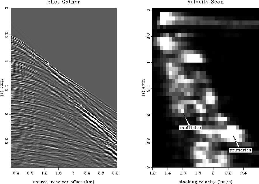The data are significantly contaminated with free-surface and water-bottom multiples which makes identification of the primary reflections difficult. Careful preprocessing will be necessary to recover the correct amplitudes on the primary reflections.

The well-log data contain depth, P-wave velocity, S-wave velocity, density, and Poisson's ratio for two wells (well A and well B) which are approximately 9.5 km apart. Figure int-ann shows the smoothed interval velocities and densities for both wells as a function of depth.

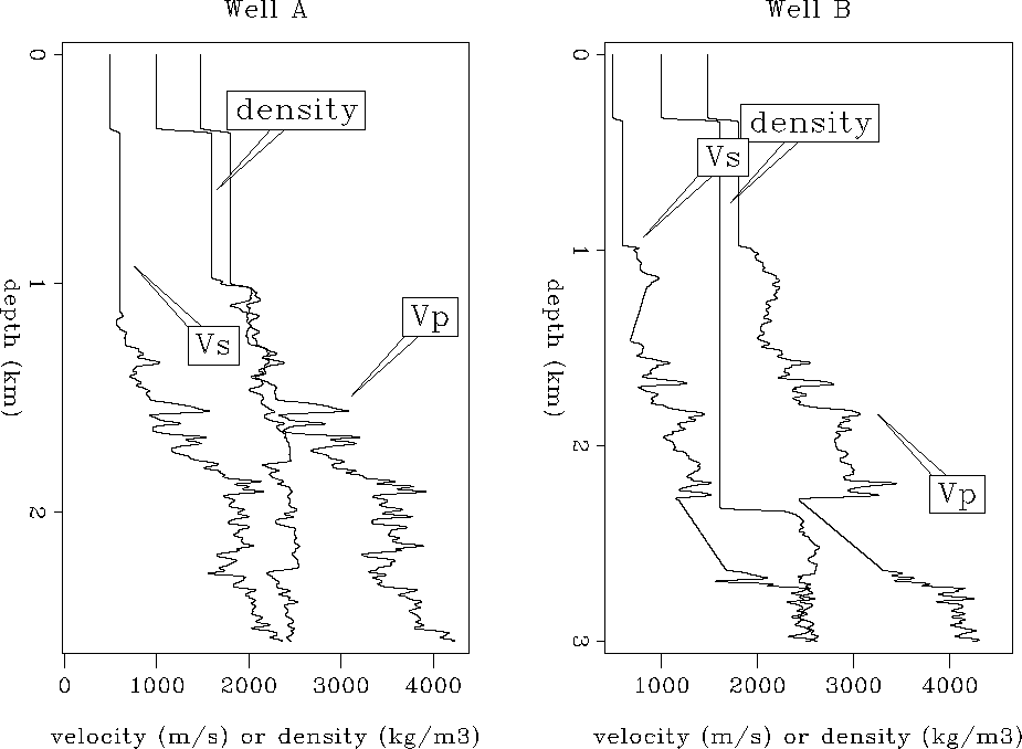As the well-log information starts from a depth of approximately 1000 meters, it does not include the shallow part of the marine sediments. The seismic properties in this zone were therefore determined based on first order approximations. The P-wave velocity in these sediments was assumed to be around 1.8 km/s, and the density was assumed to be 1.6 g/cc. Determination of an average Poisson's ratio over the entire logged depth interval yielded an S-wave velocity of approximately 0.6 km/s in the shallow sediments. The water layer was characterized by a P-wave velocity of 1.48 km/s and a density of 1.0 g/cc. While the well-log information for well A was nearly continuous for the given depth range, the data base for well B included large zones of missing velocity or density information. For both wells, missing values were approximated using linear interpolation.

Converting the interval velocities to rms-velocities yielded the velocity functions shown in Figure rms-ann. Within the first 2 seconds, the velocities obtained from well A and well B are fairly similar. At later times, the rms-velocities calculated for well B tend to be lower than those for well A. However, comparison with the interval velocities shows that the most significant deviation occurs for the linearly interpolated values after 2.4 seconds. This indicates that the velocities obtained by linear interpolation might be slightly underestimated.

The petrophysical data base indicates lithology and fluid content of both wells as a function of depth. It contains the volume fractions of dry clay, bound water, coal, quartz, calcite, parallel pores, oil, gas, and water.

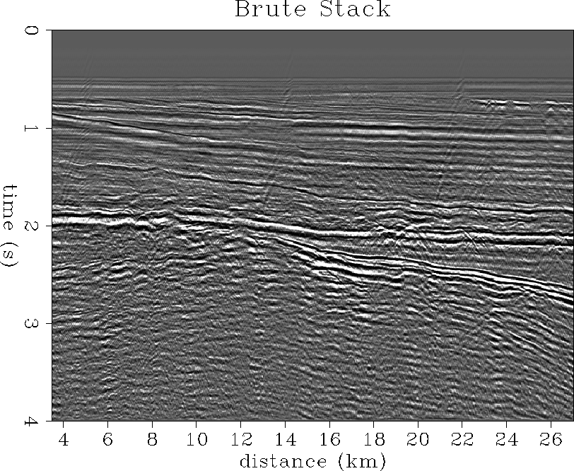
A brute stack To get a preliminary idea of stucture in the area, we made a brute stack of the Mobil AVO data, as shown in Figure

. The raw data were bandpassed and decimated from a 2 ms to 4 ms sampling interval. To speed parameter optimization, only the first four seconds of every second shot were stacked to yield a 25 m midpoint-spaced stacked section covering the full 25 km line length. The data were slightly preprocessed prior to stacking, including an outer mute at 1.3 km/s with a 200 ms linear time ramp, and a time-varying geometrical spreading correction. The CMP gathers were NMO-corrected with a single Vrms(t) function obtained by averaging the rms velocity functions from wells A and B, which are shown in Figure

The stacked section shows that the structure is fairly mild in this field, except for the basement unconformity below 2 seconds. The stack has suppressed the multiple reflection energy fairly well except near the water bottom, which indicates that most of the multiples are caused by the free surface. The two target horizons are at about 1.5 and 2.0 seconds respectively.

Receiver sensitivity varies along the cable, similarly the source strength varies from shot to shot. In order to perform a precise AVO analysis, we have estimated the source and receiver amplitude responses, and compensated the traces accordingly.

The original amplitude function has been obtained by summing all the amplitudes of the traces over the time axis. We have assumed a simple amplitude model where receiver amplitudes are constant for all shot locations at a given hydrophone position in the cable. In order to estimate the corrections that have to be applied to the data, we first removed the global trend in both receiver and shot directions. This was done by least-squares fitting a linear function in the shot direction and the exponential of a quadratic function in the offset direction ().

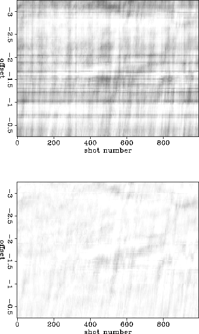The upper plot in Figure stripes shows the amplitude plane after removal of the global trend. On the grey background, horizontal and vertical stripes are visible. The horizontal stripes correspond to receivers stronger or weaker than the general tendency. The vertical stripes correspond to varying pressure shots.

We have then estimated the correction coefficients by stacking the amplitude plane separately in both offset and shot direction after removal of the global trend. On the lower plot in Figure stripes, the stripes have been eliminated by applying the correction coefficients in both direction.

MULTIPLE REFLECTIONS One of the challenges of the Mobil AVO dataset is the presence of a large amount of multiple energy on the prestack gathers, as indicated by the shot gather and velocity scan of Figure

. We intend to both 1) suppress multiple energy and recover primary reflection AVO responses in order to perform AVO analysis, and 2) use the primary and multiple reflection data simultaneously to measure and analyze AVO. Stew Levin has also urged Mobil to provide participants with a copy of their preprocessed data so that those interested in prestack inversion can get rolling quickly, leaving the subject of multiples for concurrent research. We briefly discuss several avenues we are going to pursue.

Radon transform From personal communication, we gather that Mobil has used a form of parabolic Radon filtering () with fair-to-good success in attenuating the multiple energy. We are working with the ProMAX Radon Filter module to try to achieve a similar result. Current limitations of the ProMAX module are making tests on synthetic seismograms slow going. We are currently using a CSM SU utility to facilitate the split/merge functionality needed.

$\mbox{\protect\boldmath$L_2$}$ velocity-transform pairs We have much practical experience in computing stacking velocity scans, and can use that expertise to optimally separate the multiple and primary reflection trends in velocity space. The algorithm that achieves the previous goal is the forward velocity transform. An example of the velocity transform space is shown in the scan of Figure

. Additionally, we have gained some insight in how to code adjoint and least-squares pseudo-inverse algorithms, given a forward transform code. We plan to use an enhanced forward velocity transform, its adjoint and its pseudo-inverse to suppress multiples while recovering primary reflection AVO amplitudes. This method builds upon previous work by Thorson and Harlan , and can be related to a generalized hyperbolic Radon transform multiple-suppression scheme.

Wave-equation multiple suppression For the purpose of AVO analysis, perhaps the best tool for cleaning up prestack records contaminated by multiples is the Delft surface-related multiple elimination algorithm of Verschuur . We are developing the tools needed to implement this algorithm and, as discussed in the next subsection, hope to employ them not just as a multiple suppression algorithm, but also as an AVO estimation tool.

Migrating multiples One of our goals is to apply the precept that multiples are data. We already know from Jon's Overlay program () that multiple reflections can significantly increase the precision of velocity and traveltime estimates for NMO. We also believe they can be used to increase the precision and reliability of amplitude versus angle (AVA) measurements on prestack data. We think this can be accomplished by ``migrating the multiples'' as has been previously suggested at Delft () and the Colorado School of Mines (). We believe that the surface-related multiple elimination process can be adapted to build an AVA estimate from free-surface multiple reflections. Even if such proves too grandiose for the time frame of the project, the ability to suppress free-surface multiples is in itself a desirable target. In another paper in this report, Yetmen Wang and Stew Levin develop and discuss some of the machinery they think is needed for this purpose.

There are several reasons why we are interested in building depth models for the Mobil AVO data. We will use the models to test our multiple suppression schemes in terms of recovering primary reflection AVO. We have constructed a 1-D elastic model in order to compute a full-waveform elastic CMP gather with and without free-surface multiples. We have also constructed an idealized 2-D depth model for generation of more sophisticated elastic finite-difference shot gather data. Finally, we would like to build a realistic 2-D depth model to compute Kirchhoff Green's functions for depth migration and to test wave-equation inversion schemes.

Haskell-Thompson 1-D modeling We constructed a 1-D elastic model to test our multiple suppression methods. Each layer is characterized by the constant elastic parameters P-velocity, S-velocity and density, based on the well-logs and the paper time-migrated section, which was provided by Mobil and is not shown here. We generated two CMP gathers, one with and one without free-surface multiples, using the Haskell-Thompson reflectivity propagator-matrix method.

A 1-D elastic model The model is based upon data from the well-logs, and the time-migrated section. The sea bottom depth was estimated from the time-migrated section and fathometer readings to be about 340 m in depth. Nine reflection events, including the sea bottom were picked from the time-migrated section and converted to depth using the well-log rms velocity function from well-log A (Figure

). We smoothed the well-log values for P-velocity, S-velocity and density at well A. In the zones where no data were given, we had to choose discontinuity jumps in the physical parameters. In the zones where data were available, there was a reasonable agreement between the major jumps in the physical parameters of the smoothed well-log values and the reflectors picked by hand from the time-migrated section (Figure

). We chose constant velocity and density values from the smoothed logs for each layer in our 1-D model. The model parameters are given in Table 1.

**Table 1:** The 1-D elastic model for Haskell-Thompson seismograms.
Depth (m)	Vp (m/s)	Vs (m/s)	$\rho$ kg/m³
340	1480		1000
540	1780	550	1600
690	1880	590	1850
935	1920	615	1900
1395	2030	640	2100
1795	2500	985	2170
2030	3000	1320	2400
2265	3620	1940	2280
2560	3450	1840	2450
--	3760	2136	2350

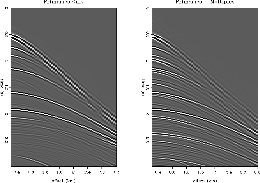
Haskell-Thompson seismograms Using the 1-D elastic model described above, we generated elastic seismograms with a Haskell-Thompson reflectivity matrix propagator method, as reviewed by Aki and Richards (1980, p.163). The goal was to generate one ``primary-reflection'' CMP gather with no free-surface effects, and one CMP gather with primaries plus free-surface multiples. We plan to test the amplitude response of our multiple suppression schemes by processing the CMP with free-surface multiples and comparing how well we can recover the primary reflections, both kinematically and dynamically in terms of original AVO values.

Figure

shows the two CMP gathers. The seismograms were generated with a zero-phase Ricker wavelet having a dominant frequency of 20 Hz. The 50 m receiver spacing and near-to-far offset values match the survey geometry of the Mobil marine data. Each CMP consists of 60 traces with a 4 ms sample interval. Comparing the right and left panel of Figure

suggests that the free surface causes a rich multiple train of events which contaminates the primary reflections. Interestingly, some PSP conversions are evident in the left panel, especially at 2.75 s, which are masked by multiples in the right panel. A preprocessing scheme would score a perfect mark on our multiple suppression test if the processed version of the right panel matched the left panel.

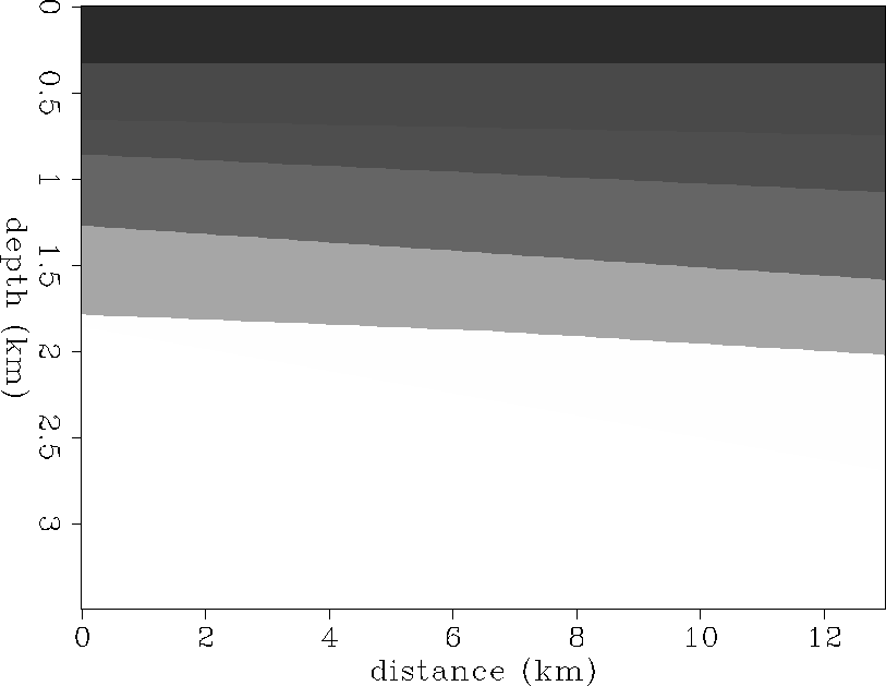
In order to be able to test more sophisticated processing methods and to obtain more realistic modeling results with regard to the present structure, we created a two dimensional model. Using an elastic finite-different modeling program developed by Karrenbach , two shot gathers were generated to simulate both the primary reflection signals and the reflection signals which include multiple energy.

In order to create the 2-D model, we first constructed a GOCAD representation of the reflection interfaces. Several major reflectors, including the seafloor, were identified in the time-migrated section along a horizontal distance of 13 km enclosing both well-log locations. Using the rms velocity functions for well A and B (Figure rms-ann), they were converted to depth and then transformed to GOCAD surfaces. These GOCAD surfaces served as an input for a 3-D gridding program () in which the third dimension was adjusted to only one grid point. As part of the gridding process, the P-wave velocities, S-wave velocities and densities of the individual domains, bounded by the surfaces, had to be specified. We assumed constant velocities and density in each layer. These parameters were extracted from the averaged information given by wells A and B. The starting depth d₀ of each reflector, its P-wave velocity, S-wave velocity and density is given in Table 2. The output of the gridding program results in a two dimensional velocity and density model. The P-wave velocity model is shown in in Figure model.

**Table 2:** Model parameters for the 2-D model.
d₀ (m)	v_p (m/s)	v_s (m/s)	$\rho$ (kg/m³)
333	1480		1000
660	1800	570	1600
861	1850	650	1650
1275	2100	790	1800
1719	2550	1200	2100
1862	3200	1600	2300
3500	3600	1800	2400

From the 2-D model, two synthetic shot gathers were generated using a finite-difference modeling approach (). An absorbing surface was incorporated to produce primary reflection energy, while a free-surface condition was used to produce multiple reflection energy. The result of this finite-difference modeling can be seen in Figure findiff.

The gathers contain 60 traces with a sampling interval of 2 ms and a receiver spacing of 25 meters. The near- and far-offset values were adjusted to approximately those of the Mobil data set. Both gathers were corrected for a time-varying spherical divergence. Comparing the gathers, the different effects of the two surface conditions are obvious. While the absorbing surface resulted in a ``clean'' gather containing mainly the primary energy, the gather produced by the free-surface condition is heavily contaminated with free-surface multiples which are masking the primary signals. While some of the primaries can still be identified by comparing the two shot gathers, others overlap with multiples resulting in a significant change in the signals.

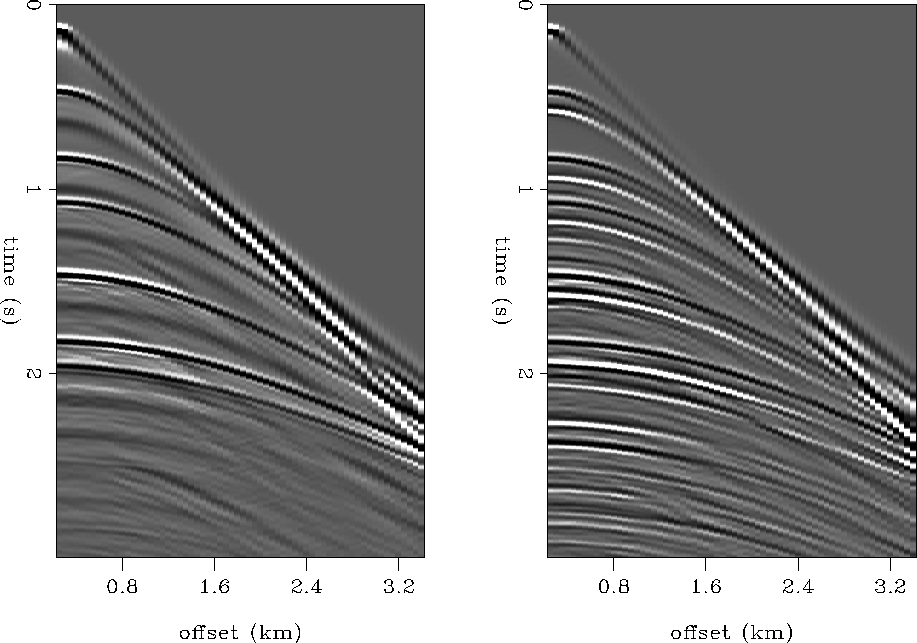These synthetic shot gathers will be used to test the different processing schemes for measuring the true AVO on the primary reflections. Both suppression or incorporation of the interfering multiple energy in the processing should produce the multiple-free synthetic shot gather from the one contaminated with multiples.

After careful true-amplitude preprocessing and multiple suppression, the data will be suitable for AVO analysis and impedance inversion. Subsequently, we will try to relate the estimated seismic parameters to lithology and pore fluid content by developing AVO indicators in conjunction with rock physics analysis and the Mobil petrophysical database.

The simplest approach is to first perform a linearized parameter inversion on unmigrated amplitude-corrected CMP gathers. Ecker and Lumley showed an example of this on methane hydrate AVO data. In a more sophisticated analysis, a Kirchhoff wave-equation elastic impedance inversion will be attempted. The basis of this technique was described by Lumley and Beydoun , and was applied in a gas reservoir study by Lumley and in a recent methane hydrate analysis by Ecker and Lumley . Since the field structure is not complicated, we also expect to make a meaningful comparison of time and depth migration/inversion results on the Mobil data.

Another approach is to analyze the angle-dependent reflectivity image obtained by imaging with wavefront synthesis. This technique was described by Ji and was tested on the Marmousi dataset. Unlike the Marmousi data, the simple structure on the Mobil data should provide more interpretable angle-dependent reflectivity image.

In summary, we have given an overview of our AVO project, from preliminary results to planned research strategy. We expect to participate in Mobil's AVO review workshop in London this summer, and at the special SEG AVO workshop in Los Angeles this October. We plan to harness our combined technical skills and field-data expertise in order to solve some of the challenging problems presented in the Mobil AVO dataset as part of an ongoing SEP project.

We would like to thank Bob Keys of the Mobil Exploration and Production Technical Center for providing SEP with the Mobil AVO dataset, and visiting us to discuss our mutual AVO research interests.

An AVO analysis project

ABSTRACT