Next: 3-D SYNTHETIC EXAMPLE
Up: Cole: Statics estimation by
Previous: Interpolation
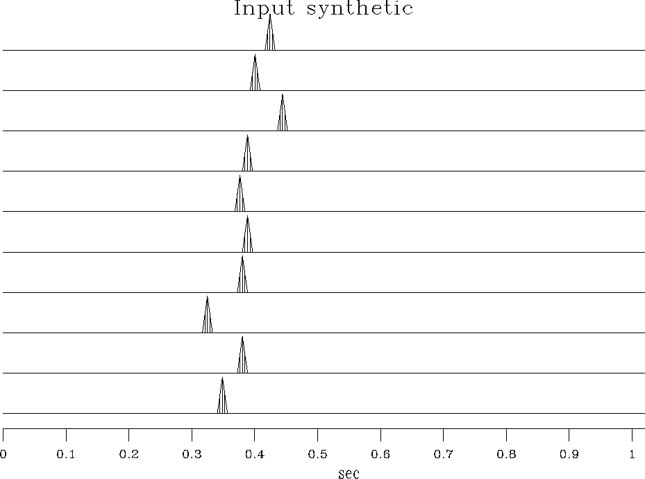
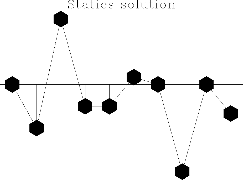
Figure ![[*]](http://sepwww.stanford.edu/latex2html/cross_ref_motif.gif) shows a 2-D synthetic example. A dataset containing a
single dipping plane wave (apparent velocity 3 km/sec) has had applied
to it the statics solution shown in Figure .
The trace spacing is 20 meters and the time sampling interval
is four milliseconds.
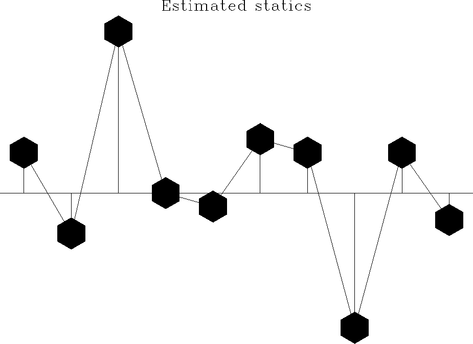
A single dip estimation was performed at the middle receiver,
using all ten neighboring traces.
The statics estimated by the algorithm are shown in Figure .
While the relative shifts are correct, there is a time shift
that reflects the presence of a DC bias in the random statics
values that I chose to apply. This bias has been removed from the
solution.
shows a 2-D synthetic example. A dataset containing a
single dipping plane wave (apparent velocity 3 km/sec) has had applied
to it the statics solution shown in Figure .
The trace spacing is 20 meters and the time sampling interval
is four milliseconds.
A single dip estimation was performed at the middle receiver,
using all ten neighboring traces.
The statics estimated by the algorithm are shown in Figure .
While the relative shifts are correct, there is a time shift
that reflects the presence of a DC bias in the random statics
values that I chose to apply. This bias has been removed from the
solution.
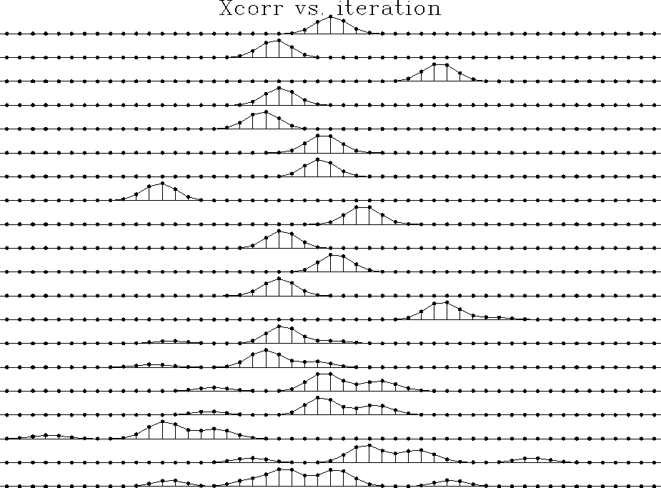
The crosscorrelation functions for each receiver for the first
two iterations are displayed in Figure .
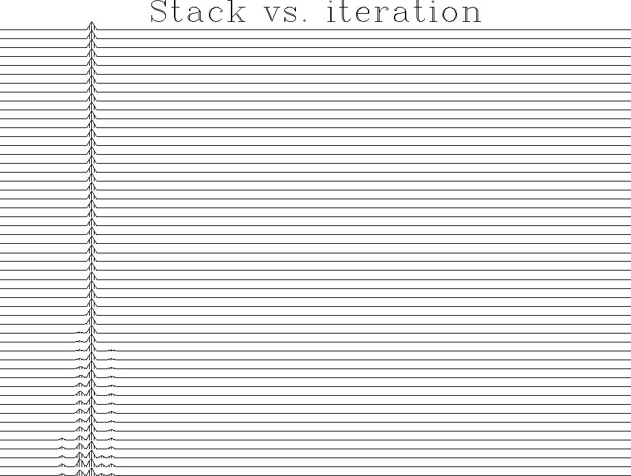
Figure shows the improvement in the stack over
the course of the first two iterations. Actually a single
iteration was sufficient in this simple case.
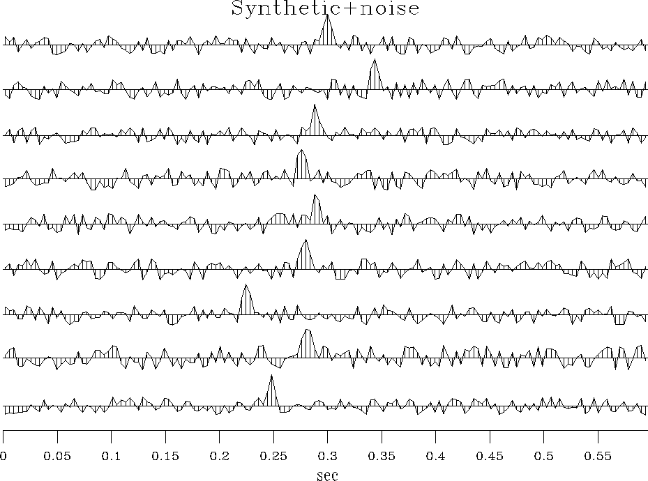
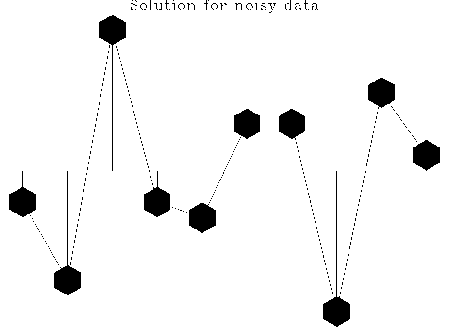
In Figure , random noise has been added to the synthetic.
The statics solution in Figure is similar to the
previous one, but there is
a clear linear trend in the solution that represents poorly estimated
long wavelength statics. These become even more problematic on a
larger 3-D example in the following section.
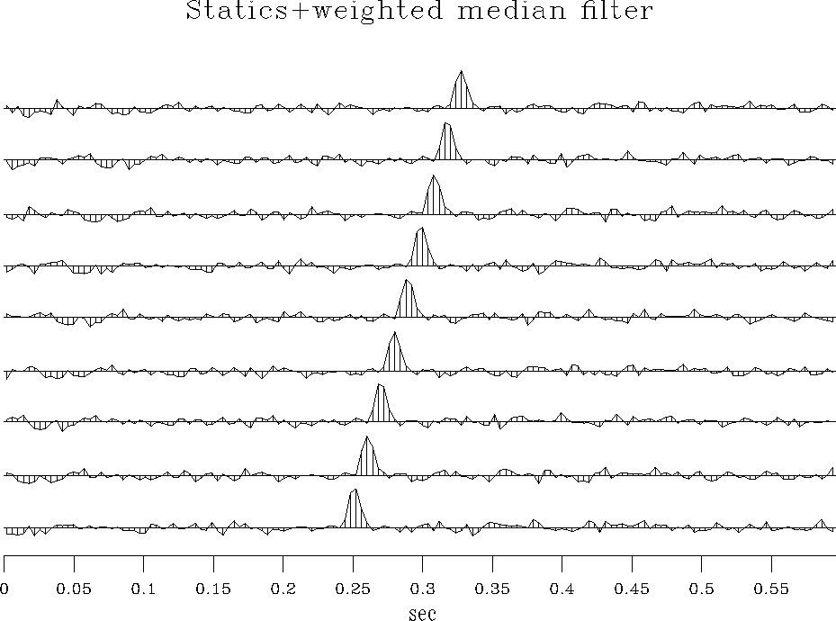
Figure shows the result of applying the statics to the
noisy data. After statics application, the data have been interpolated
onto the original recording geometry by a local slant stack at the
correct dip. A median filter has been used in place of the straight
stack, and the output has been weighted by the semblance. This nonlinear
weighting enhances the coherent signal. Because a single time window was
used in this example, some alignment of noise along the same dip can
be seen.
syn2d
Figure 1 A 2-D synthetic example. The statics shown in Figure have been applied to a dataset containing a single dipping plane wave.

statin2d
Figure 2 Random statics applied to create the data in Figure .
|
|  |
statout2d
Figure 3 Statics solution estimated by the algorithm.
|
|  |
stak2d
Figure 4 Iterative improvement of the local slant stack. The bottom trace is the initial stack. Each additional trace represents the result of updating the static solution for a single receiver. The first ten traces correspond to the first iteration of the algorithm, the second ten to the second iteration.


 xcor2d
Figure 5 Display of crosscorrelations for the first two iterations. From bottom to top, the first ten traces are the crosscorrelations for the ten different receivers for iteration one, the next ten for iteration two.
noise2d
Figure 6 Synthetic with random noise added.
noiseout2d
Figure 7 Noisy synthetic after application of statics, followed by interpolation onto the original grid, using a median filter and semblance weighting. A single semblance computation window was used for the entire trace, and some alignment of the noise can be seen.
noisestat2d
Figure 8 Statics solution for noisy
data. Compared with Figure , here there is a trend
from lower left to upper right, indicating
that the long wavelength statics have not been determined well.
|
|  |
Next: 3-D SYNTHETIC EXAMPLE
Up: Cole: Statics estimation by
Previous: Interpolation
Stanford Exploration Project
11/16/1997