


The extension of f-x prediction to three-dimensions is more difficult than
that of t-x prediction.
For each frequency,
instead of a prediction along a vector,
the prediction
of a set of complex numbers within a plane is required.
For the examples of three-dimensional f-x prediction shown here,
we used a complex-valued two-dimensional
filter calculated
with a conjugate-gradient routine for each frequency.
While other techniques for computing this filter
exist,
they should produce similar results.
The advantage of our approach is that the huge
matrix ![]() used to describe
the three-dimensional convolution of the filter with the
data does not need to be stored, and the inverse of
used to describe
the three-dimensional convolution of the filter with the
data does not need to be stored, and the inverse of ![]() does not need to be computed,
which simplifies the problem
significantlyClaerbout (1992a).
does not need to be computed,
which simplifies the problem
significantlyClaerbout (1992a).
The shape of the two-dimensional filter used to predict numbers in a two-dimensional frequency slice has the form
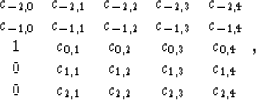 |
(9) |