


For AVO analysis, the most widely used approximation of the reflection coefficient was derived by Shuey 1985 in the following equation:
| |
(4) |
where ![]() is the incidence angle, R0 the reflectivity for zero
incidence, and G a quantity related to elastic parameters. This
linearization defines a framework within which seismic amplitudes must fit.
Conventionally this formula can be directly applied to an NMO-corrected CMP
gather. For every sample point, amplitudes are used to compute R0
and G through a linear regression. The series R0(t)*G(t)
provides a useful section for AVO analysis. In this section, positive
amplitude indicates amplitude increasing with offset, and negative amplitude
indicates amplitude decreasing with offset.
is the incidence angle, R0 the reflectivity for zero
incidence, and G a quantity related to elastic parameters. This
linearization defines a framework within which seismic amplitudes must fit.
Conventionally this formula can be directly applied to an NMO-corrected CMP
gather. For every sample point, amplitudes are used to compute R0
and G through a linear regression. The series R0(t)*G(t)
provides a useful section for AVO analysis. In this section, positive
amplitude indicates amplitude increasing with offset, and negative amplitude
indicates amplitude decreasing with offset.
With data from the ![]() domain in each CMP gather, we can do
the AVO analysis directly according to equation (4), after some preprocessing for
amplitude correction. Because we already know the value of p for each trace
and the interval velocity in depth, we can calculate the
domain in each CMP gather, we can do
the AVO analysis directly according to equation (4), after some preprocessing for
amplitude correction. Because we already know the value of p for each trace
and the interval velocity in depth, we can calculate the
![]() in equation (4)
directly from
in equation (4)
directly from
| |
(5) |
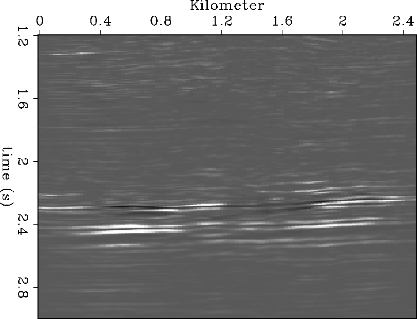
Owing to the prestack migration, the seismic events were moved to the correct position, and more accurate amplitude was recovered. Figure 8 shows the R0*G section after linear regression of the migrated CMP gathers. This section displays bright spots (at 2.2 seconds and 1.8 Kilometers), which is similar to those in Figure 13 of Lumley's paper 1993. They indicate a known gas producing reservoir.
 |


