|
model
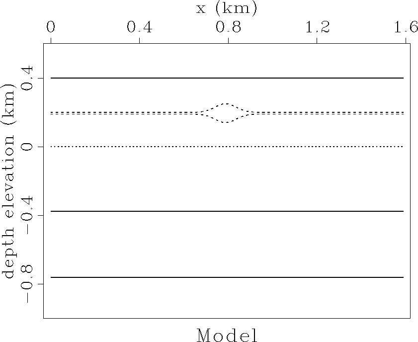
Figure 1 Two horizontal reflectors at |  |
|
model
Figure 1 Two horizontal reflectors at |  |
Synthetic data are generated using two Kirchhoff modeling
programs.
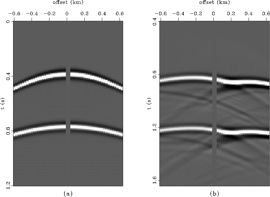
I first generate constant velocity synthetic shot gathers
(Figure 2a) using a
constant offset migration and modeling program similar to the program
described in a previous report Bevc and Claerbout (1993).
These synthetic gathers are generated at a depth of ![]() (Figure 1).
The synthetic data are then upward continued to an elevation of
(Figure 1).
The synthetic data are then upward continued to an elevation of ![]() using a data parallel Kirchhoff datuming
algorithm Bevc (1993).
The upward continuation is performed in three steps, using constant
velocities in each step. The first upward continuation transforms the data
from the flat surface at
using a data parallel Kirchhoff datuming
algorithm Bevc (1993).
The upward continuation is performed in three steps, using constant
velocities in each step. The first upward continuation transforms the data
from the flat surface at ![]() to the Gaussian surface
to the Gaussian surface ![]() .
The data are then upward continued with a low velocity to the next Gaussian
surface. The complete synthetic data set is generated by upward continuing
the data to the level surface at elevation
.
The data are then upward continued with a low velocity to the next Gaussian
surface. The complete synthetic data set is generated by upward continuing
the data to the level surface at elevation ![]() .
.
The effect of the low velocity perturbation can be seen in Figure 2b as a timing and focusing anomaly. Because of the focusing effect, a static shift of the data is not adequate to correct for the velocity perturbation. As the shot number increases, the anomaly moves from right to left across the gathers. There are some artifacts in the synthetics because of data truncation effects and the rapid undulation of the Gaussian boundary.
 |